My clients sometimes ask for help with building Excel dashboards, so they can present a summary of their data to their customers and co-workers.
In a dashboard, you want to make the best use of limited space, and only show key information. For example, instead of showing all the sales data, you can show just the highest and lowest values.
MIN and MAX Functions
It’s easy to pull the top and bottom values from a list, by using the MIN and MAX functions. It’s a little trickier though, if you want to show the high and low amounts for a specific product in a long list.
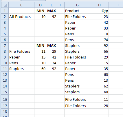
In this example, I want to calculate the MIN and MAX for each product, then put that information on the dashboard
Create a MIN IF or MAX IF formula
There’s no built-in MINIF or MAXIF function, but you can use MIN or MAX with the IF function, to create your own. The steps are shown in the video, at the end of this article.
First, to get the minimum quantity sold for File Folders, the array formula in cell D8 is:
=MIN(IF($G$2:$G$17=C8,$H$2:$H$17))
After you type the formula, press Ctrl + Shift + Enter, so it is array entered.
The same technique is used in cell E8, with MAX, instead of MIN:
=MAX(IF($G$2:$G$17=C8,$H$2:$H$17))
Excel Dashboard Course
If you’d like to add dashboard skills to your Excel tool kit, I recommend the upcoming Excel Dashboard Course offered by Mynda Treacy from My Online training Hub. Mynda is an accountant, and her dashboards focus on the numbers, not the fluff.
There are 9 sessions in the course, with video tutorials that are short and to the point. They cover the key steps and features, and you can practise the techniques in the sample files. Replay the videos as often as you need, for up to 12 months. The course includes 6 weeks of support from Mynda, so you can post questions, read comments, and ask her to review your completed dashboard.
This course is not for Excel beginners, because the fast pace could be overwhelming. Lots of material is covered, very quickly. And, if you’re already a dashboard expert, you won’t need this course. It’s designed for Excel users who are beyond the basics, and who enjoy learning by seeing a demo, then practising the new skills.
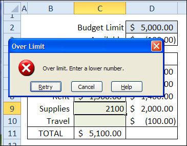
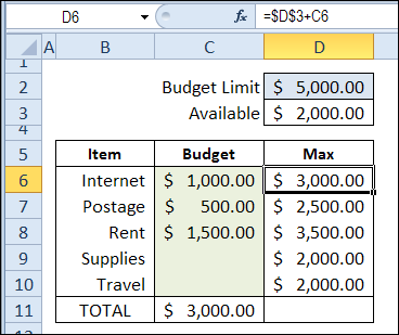
In the new version, I’ve added a few more features, to help you fill in the correct amounts.
Below the Budget Limit, in cell D3, you can see the amount that hasn’t been added to the budget yet.
In column D, you can see the maximum amount that can be entered in each row, based on the entries in other rows. This makes it easier to adjust individual items, while you finalize the budget.
data validation in cell D2 limits budget amount
And remember, data validation isn’t foolproof, so you’ll still have to check those budgets, to make sure nobody is trying to get a little extra!
Download the Sample File
To see the formulas, and test the data validation, you can download the sample budget from my Contextures website.
Go to the Sample Excel Files page, and in the Data Validation Section, look for DV0058 – Limit Budget Entries with Data Validation.
Watch the Budget Limits Video
To see the steps for setting up the data validation and formulas, to set the budget limits, you can watch this short video tutorial.
Last week, a client sent me a workbook that I created for them a couple of years ago. They were having problems with it, even though things had been going smoothly since we first installed it.
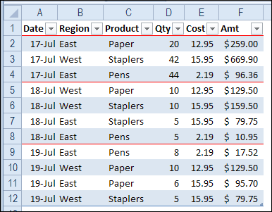
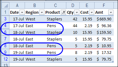
Recently, I heard from Lon, who liked the tip about red line borders. But Lon noticed a problem – the line didn’t always show if the list was filtered.
For example, if we filter the Product column, to hide Paper, the red borders for some of the dates disappear.
Lines Disappear in Filtered Lists
I hadn’t noticed the problem, because my list is usually filtered by date, to show only the latest month’s data. Since the conditional formatting is based on the date column, it would continue to work correctly.
But we can change the conditional formatting, so it works in a filtered list.
Change the Formula for Filtered Lists
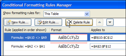
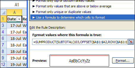
To make the conditional formatting work in a filtered list, we can’t use the original formula, which was
=$A1<>$A2
That formula just compares each date to the date above it, and doesn’t care if the rows are hidden or visible.
Instead, we’ll use a formula that was created by Laurent Longre. It lets you work with visible rows after a filter. For information on this formulas, read the Power Formula Technique section, in this article at John Walkenbach’s web site: Excel Experts E-letter
Here is the much longer formula that we can use, to compare dates in the visible rows only.
Note that there are two minus signs in front of the last open bracket – it’s not a long dash.
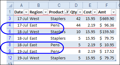
Date Separator Lines Show When Filtered
With the new formula, the red lines separate the dates, even if the list is filtered. In the screen shot below, the Product column is filtered to hide Paper, but the date line for July 18th shows up.
And you can download the sample file used in this blog from the Contextures Sample Excel Files page. In the Conditional Formatting section, look for CF0004 –Conditional Formatting in Filtered List. The zipped file is in Excel 2007/2010 format, and contains no macros.
Stephan emailed me recently, and asked what books I’d recommend for an advanced beginner and for an intermediate user.
On the Contextures website, I’ve got a list of Excel books. They range from books for absolute beginners, to specialized books on statistics and financial modelling.
Book Suggestions
Here are the advanced beginner books that I suggested to Stephan – do you agree with these choices?
You might find these at your local library, or a nearby bookstore
Microsoft Excel 2010 Step by Step; Curtis Frye; ISBN: 0735626944; 480 pages; 2010; US$29.99
Slaying Excel Dragons: A Beginners Guide to Conquering Excel’s Frustrations and Making Excel Fun; Mike Girvin, Bill Jelen; Holy Macro! Books; ISBN: 978-1615470006; 532 pages; 2011; US$29.95
If you’re book shopping online, before you buy an Excel book on Amazon, use the “Look Inside” feature, if available, to see what the writing style is like, and check the table of contents.
The quick peek will give you a general overview of the book, and could help you decide if the book is right for you.
Read the Reviews
The customer reviews can be helpful too – both the negative and positive ones. Sometimes another person doesn’t like a book because it’s not for absolute beginners, and that might be a positive thi ng for you
. And there’s always the possibility that some of the glowing reviews were written by the author’s mother or friends! 😉
If you can get to a bookstore, you can flip through the Excel books there, and head home with a few that you like.
It sometimes costs a bit more than shopping online, but it’s worth it, to find the books that are best suited to your needs and learning style.
Use INDEX and MATCH together, for a powerful lookup formula. It’s similar to a VLOOKUP formula, but more flexible — the item that you’re looking for doesn’t have to be in the first column at the left. Watch the video to see how it works (there are written instructions too), and download the sample workbook to follow along. Continue reading “Check Multiple Criteria with Excel INDEX and MATCH”
In a complicated Excel file, you might end up with several code modules, and it’s easy to lose track of what’s connected to what. Here’s how you can document your Excel VBA procedures.
You spend time setting up your worksheets exactly the way you want them – the headings are frozen at the top of the screen, gridlines are turned off, and a few other customizations are made. Beautiful!
When you build an Excel tool or template, it’s rare that you’re ever really finished building. There’s always something that would make the tool a little better, either for your own use, or for your customers.
And that’s the case with the Excel worksheet data entry form, which I’ve just updated again.
In the latest version, I fixed an issue with the navigation. Thanks to Travis, who let me know about the problem.
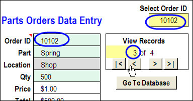
Now, when you move to a different record with the arrow buttons, the Order ID selector also updates.
You can see the Order ID, the Order ID selector, and the record number, circled in the screen shot below.
Order ID, Order ID selector, record number
Add or Update
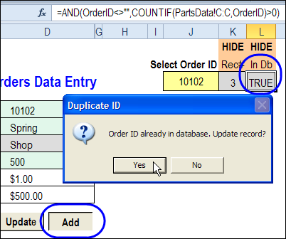
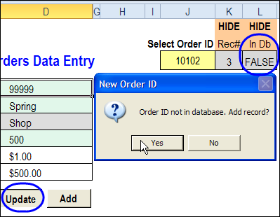
The other enhancement is a database check, when you click the Add or Update button. In a hidden column, a COUNTIF formula counts the selected Order ID occurrences in the database.


 Stephan emailed me recently, and asked what books I’d recommend for an advanced beginner and for an intermediate user.