A while ago, I showed you how to add a red border at the top of a row, when a new date starts in a list.
You can read those instructions here: Separate Excel List with Automatic Lines.
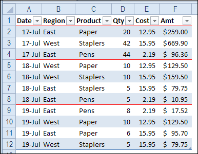
Conditional Formatting Problem
And if you’re using this technique, remember the painful lesson that I learned – don’t copy and paste within a table that has conditional formatting.
You could end up with an Excel 2010 Conditional Formatting Nightmare. And nobody wants that!
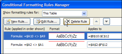
Lines Disappear in Filtered Lists
Recently, I heard from Lon, who liked the tip about red line borders. But Lon noticed a problem – the line didn’t always show if the list was filtered.
For example, if we filter the Product column, to hide Paper, the red borders for some of the dates disappear.
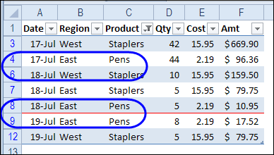
I hadn’t noticed the problem, because my list is usually filtered by date, to show only the latest month’s data. Since the conditional formatting is based on the date column, it would continue to work correctly.
But we can change the conditional formatting, so it works in a filtered list.
Change the Formula for Filtered Lists
To make the conditional formatting work in a filtered list, we can’t use the original formula, which was
=$A1<>$A2
That formula just compares each date to the date above it, and doesn’t care if the rows are hidden or visible.
Instead, we’ll use a formula that was created by Laurent Longre. It lets you work with visible rows after a filter. For information on this formulas, read the Power Formula Technique section, in this article at John Walkenbach’s web site: Excel Experts E-letter
Here is the much longer formula that we can use, to compare dates in the visible rows only.
=SUMPRODUCT(SUBTOTAL(103,OFFSET($A$1:$A2,ROW($A$1:$A2)
-MIN(ROW($A$1:$A2)),,1)), –($A$1:$A2=$A2))=1
Note that there are two minus signs in front of the last open bracket – it’s not a long dash.
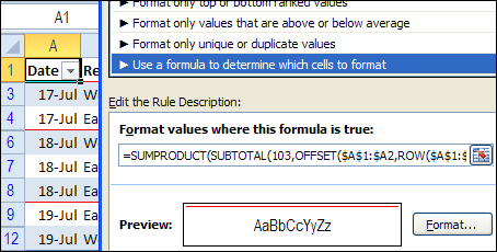
Date Separator Lines Show When Filtered
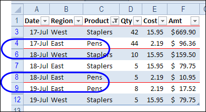
With the new formula, the red lines separate the dates, even if the list is filtered. In the screen shot below, the Product column is filtered to hide Paper, but the date line for July 18th shows up.
Download the Sample File
There is another example of this type of formula on my Contextures website – Count Visible Items in a Filtered List.
And you can download the sample file used in this blog from the Contextures Sample Excel Files page. In the Conditional Formatting section, look for CF0004 – Conditional Formatting in Filtered List. The zipped file is in Excel 2007/2010 format, and contains no macros.
_________________
