
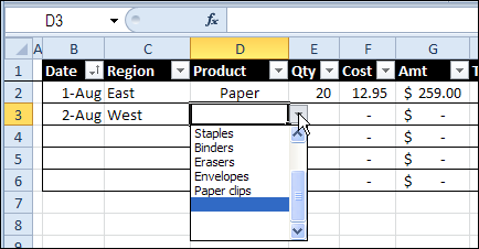
To make data entry easier, you can create a drop down list of items in a worksheet cell. Then, instead of typing a product name in an order list, you can select a valid product name from the list. Sometimes the Excel drop down opens at end of the list, instead of the top. Here’s how to fix that problem.
Update Specific Pivot Tables Automatically
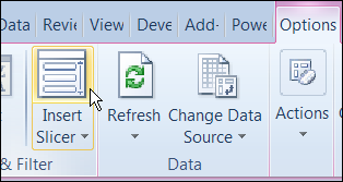
In Excel 2010, you can use Slicers to change multiple pivot tables. However, you might be working in an earlier version of Excel, or you don’t have room for Slicers on your worksheets.
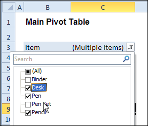
Instead of Slicers, you can use programming to update multiple pivot tables automatically. In previous posts, I’ve shown how you can select items in one pivot table’s Report Filter fields, and the Report Filter fields for pivot tables on the other worksheets will change to the same selections.
Specific Sheet and Pivot Tables
Jeff Weir has written an updated version of the code, which runs much faster than the previous version. You’ll notice the speed difference especially if you’re working with larger pivot tables.
Also, in this version of the code, you can specify:
- any sheets you DON’T want the macro to check
- any specific pivot tables that you DON’T want the macro to synchronize.
For example, only update the pivot tables on Sheet1 and Sheet2, and ignore PivotTable2 on Sheet1.
[Update: Sept 20, 2012] Jeff has made the following changes to the code:
- you can now exclude particular PivotFields, plus if you change a pagefield in any pivot, the code will not only update pagefields to the same settings in other pivots but also change rowfields too.
- added basic error handling so that ScreenUpdating and EnableEvents are restored to TRUE if anything goes wrong.
Jeff is also working on a version of the code for Excel 2010, that promises to be even faster — so stay tuned for that!
[Update: June 16, 2013] Jeff has revised the code, so it uses Slicers if the version is Excel 2010 or later.
Making Code Run Faster
In the previous version of the code, it looped through each master pivot field multiple times, to determine if each pivot item is visible or hidden. The corresponding pivot item in each secondary pivot table was then set to the same setting. The code worked, but it was very slow in larger pivot tables.
The main reason that Jeff’s code is faster is that it iterates through each master pivot field just once, so it can record only the visible items into a dictionary.
Then, for each pivot field in each secondary pivot table:
- All the pivot items are made visible
- Items that are not in the dictionary’s list are hidden.
Also, speed in Jeff’s code is increased because it:
- checks to see if.AllItemsVisible = true. If it is, no need to iterate through either the master or the secondary pivot…it just makes all pivot items in the corresponding secondary pivot fields visible. The old code looped through each pivot item
- doesn’t add items to the dictionary for checking if it has already found all the visible pivot items in the master list.
Modify the Code
If you download the sample file (see instructions below), you can copy the code to your own workbooks.
- To see the code in the sample file, go to the Sales Pivot worksheet, right-click the sheet tab, and click View Code.
- Then, to see the full code, right-click on the procedure name – SyncPivotFields – and click Definition
Here is where you’ll change the sheet names in the SyncPivotFields code:

Here is the section where you’ll change the pivot table names:

Download the Sample File
To download this version of the sample file, with Jeff’s code, please visit the Sample Files page on the Contextures website.
Note: Jeff’s sample file was updated on Sept. 20, 2012, so please download the new version if you have an older copy of the file.
In the Pivot Tables section, look for: PT0029 – Change Pivot Table Fields on Specific Sheets
The file is in Excel xlsm format, zipped, and contains macros. Enable the macros when opening the file, if you want to test the code.
__________________
How to Create a Panel Chart in Excel
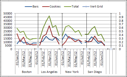
To show a concise, clear summary of data for several departments or cities, you can create a panel chart in Excel. It shows all the data in a single chart, with vertical lines separating the groups.
Edit Excel List Data in Popup Form
If you’re working with a list of data in Excel, you can use Excel’s built-in Data Form to view and edit the data.
Displaying up to 32 fields, it lets you view and edit one record at a time. You can also find and edit records, or add and delete them.
Continue reading “Edit Excel List Data in Popup Form”
Print Numbered List of Excel Comments
In Excel, there are two built-in options for printing comments. The first choice is to print them at the end of the worksheet.
For that selection, all the worksheet comments are listed in a single column, with labels to the left, as shown below.

Print As Displayed
The other option is to print comments as displayed on the worksheet. Any comment that is currently visible on the worksheet will print, exactly as they appear on screen.
If you arrange things carefully, they’ll look okay, but with closely positioned comments things will look messy.

Print a Numbered List
On my Contextures website, there is code that lets you show a number at the top right of each comment cell. These little rectangles cover up the red triangle that marks the comment cells.
This is a zoomed in view of the numbers.

Macro to Print List
There is also sample code creating a numbered list of comments on a separate sheet. Thanks to Dave Peterson for writing that!

List Comments With Merged Cells
I avoid merged cells whenever possible, and hadn’t noticed that there was a problem listing comments that are in merged cells.
Someone contacted me last week, to see if there was a way to list those comment cells once, instead of listing all the cells in the merged area.
Here’s the list, using the old code. Cells A1:D1 are merged, and they’re all listed.

New Macro for Merged Cells
So, I’ve created a new procedure in the Excel 2007 file, and added a button to the worksheet. If your worksheet has merged cells with comments, use that button, for better results in the numbered list.
The code works with merged or normal cells, and also copies the number format from the source cell.
Here is the list created by the new code. There is only one listing for the merged cell, and the Tax cell shows the number formatted as a percentage.

Download the Sample File
To download the sample file for Excel 2003 or Excel 2007/2010, go to the Number and List Comments section on the Comments programming page.
There’s sample code to add numbers, remove numbers and list the comments, and a zipped sample file that you can download.
The Excel 2003 numbering code didn’t work well in Excel 2007. The numbers didn’t appear in some boxes, and the boxes didn’t line up correctly in the cells. So if you’re using Excel 2007, be sure to download that version’s sample file
Both files contain macros, so you may get a warning when you open them. Enable the macros if you want to run the code.
_____________________________
Create an Excel Scenario Summary
Last week I updated the Excel Scenario page, and now I have added a video for the Excel Scenario Summary page. It shows the steps for creating an summary table ad a summary pivot table.
Static Reports
Unfortunately, both types of Scenario summary report are static, and they don’t update if the Scenario data changes.
Tip: If you create a Scenario Summary, be sure to date stamp it, or delete it before saving the workbook. You don’t want to keep potentially misleading data in your files.
Scenario Summary Formatting
And the Scenario Summary formatting is about as ugly as Excel gets – purple and grey.
Maybe they’ll improve that in the next version! But don’t hold your breath — I doubt that it will ever be changed.

Watch the Video
To see the steps for creating Scenario Summary, please watch this short video tutorial.
This video includes a tip for adding the Scenario command in the Excel 2010 Ribbon, so it is easy to switch between Scenarios.
More Tutorials
Here are links to 3 more Scenario tutorials, on my Contextures site:
Create and Show Scenarios – With Scenarios in Excel, you can store multiple versions of data, in the same cells
Automatically Show Scenarios – see how to use a macro to automatically show a Scenario, when you select its name from a drop down list on the worksheet
Scenarios Programming – Use these macros to create a list all the scenarios, or create new scenarios, or update the values for existing scenarios, from a list on the worksheet
______________________
Copy Code to Your Excel Workbook
You might find Excel code on this blog, or my Pivot Table blog, and want to copy it into your own workbooks.
I’ve updated my web page, Adding Code to an Excel Workbook, to show instructions for Excel 2010.
New Video
There’s a new video on that page too, that shows how to
- copy Excel code from the internet
- insert a code module in Excel
- paste the code into the module
- run the new macro
- save the file as macro enabled
Video: Copy Excel VBA Code
You can watch the new video here too, if you’d like to see the steps.
In the video, the sample pivot table code was copied from the Excel Pivot Tables blog: Change All Pivot Table Value Fields to SUM
NOTE: For the Excel 2003 version of the Copy Code tutorial, please visit: Copy Code to Excel 2003 Workbook
Modify the Code
It’s not always so simple to copy Excel code, and use it in your workbooks. You might have to modify the code, by changing worksheet names, or cell references, to match what is in your file.
For example, if you copy my code for multiple selections from an Excel drop down, you might have your data validation cells in a different column. You could change the column number in the code, as shown in the following video.
Note: This code goes on a worksheet module, instead of a regular module.
_________________
Store Multiple Values With Excel Scenarios
If you’re working on the office budget, you might be collecting data from different departments.
Or maybe you’re planning your back to school spending.
- If you get bonus at the end of your summer job, you can use some higher budget numbers.
- If the bonus falls through, you’ll need your low budget estimates.
Store Data With Scenarios
With Excel Scenarios, you can store different sets of values (in up to 32 cells) in a workbook. Then, without any programming, you can switch between the saved values.
In this example, we store budget projections for two departments. View and print one department’s budget, and then switch to the other department, all in the same cells.

Download the Sample File
To see the written instructions for creating scenarios, please visit the Excel Scenarios page on the Contextures website.
There is a sample file that you can download, to see how the Scenarios work.
Watch the Excel Scenarios Video
To see the steps for creating and showing scenarios, you can watch this short video tutorial. I also share tips for quickly naming cells, and automatically adding those names to your formulas.
sure to date stamp it, or delete it before saving the workbook. You don’t want to keep potentially misleading data in your files.
Scenario Summary Formatting
And the Scenario Summary formatting is about as ugly as Excel gets – purple and grey.
Maybe they’ll improve that in the next version! But don’t hold your breath — I doubt that it will ever be changed.
Watch the Video
To see the steps for creating Scenario Summary, please watch this short video tutorial.
This video includes a tip for adding the Scenario command in the Excel 2010 Ribbon, so it is easy to switch between Scenarios.
More Scenario Tutorials
Here are links to 3 Scenario tutorials, on my Contextures site:
Create and Show Scenarios – With Scenarios in Excel, you can store multiple versions of data, in the same cells
Create Scenario Summaries – After you create 2 or more different Scenarios in Excel, use a Scenario Summary to show an overview of the data. This is a static report that is designed to show the Scenario data at a moment in time.
Automatically Show Scenarios – see how to use a macro to automatically show a Scenario, when you select its name from a drop down list on the worksheet
Scenarios Programming – Use these macros to create a list all the scenarios, or create new scenarios, or update the values for existing scenarios, from a list on the worksheet
____________________
Interactive Excel Sample Data
There’s sample data on my Contextures website, and it’s useful for testing formulas and pivot tables in Excel.
On that page, there’s a link to a downloadable Excel file, with the same sample data. Or, you could just copy and paste the data into a workbook.
Excel Dashboard High and Low Values
My clients sometimes ask for help with building Excel dashboards, so they can present a summary of their data to their customers and co-workers.
In a dashboard, you want to make the best use of limited space, and only show key information. For example, instead of showing all the sales data, you can show just the highest and lowest values.
MIN and MAX Functions
It’s easy to pull the top and bottom values from a list, by using the MIN and MAX functions. It’s a little trickier though, if you want to show the high and low amounts for a specific product in a long list.
In this example, I want to calculate the MIN and MAX for each product, then put that information on the dashboard
Create a MIN IF or MAX IF formula
There’s no built-in MINIF or MAXIF function, but you can use MIN or MAX with the IF function, to create your own. The steps are shown in the video, at the end of this article.
First, to get the minimum quantity sold for File Folders, the array formula in cell D8 is:
=MIN(IF($G$2:$G$17=C8,$H$2:$H$17))
After you type the formula, press Ctrl + Shift + Enter, so it is array entered.
The same technique is used in cell E8, with MAX, instead of MIN:
=MAX(IF($G$2:$G$17=C8,$H$2:$H$17))

Excel Dashboard Course
If you’d like to add dashboard skills to your Excel tool kit, I recommend the upcoming Excel Dashboard Course offered by Mynda Treacy from My Online training Hub. Mynda is an accountant, and her dashboards focus on the numbers, not the fluff.

There are 9 sessions in the course, with video tutorials that are short and to the point. They cover the key steps and features, and you can practise the techniques in the sample files. Replay the videos as often as you need, for up to 12 months. The course includes 6 weeks of support from Mynda, so you can post questions, read comments, and ask her to review your completed dashboard.
This course is not for Excel beginners, because the fast pace could be overwhelming. Lots of material is covered, very quickly. And, if you’re already a dashboard expert, you won’t need this course. It’s designed for Excel users who are beyond the basics, and who enjoy learning by seeing a demo, then practising the new skills.
You can see the course details and a sample video here: Excel Dashboard Course
Registration is only open for two weeks, until August 14th, so don’t wait!
Watch the Min and Max Video
To see the steps for creating MIN, MAX, MIN IF and MAX IF formulas, please watch this short video tutorial.
_______________________________