If you’re upgrading to Excel 2010, you’ve probably noticed that the Conditional Formatting feature has changed quite a bit.
Now you can apply more than 3 rules, and there are fancy features like data bars and icon sets.
Conditional Formatting Icon Sets in Excel 2010
Intro to Conditional Formatting
On my Contextures site, I’ve updated my Intro to Conditional Formatting page, to show Excel 2010 instructions. I’ve also made a new video to show the steps n the new version of Excel.
Note: If you’re looking for Excel 2003 instructions, they’ve been moved to this page: Excel 2003 instructions.
Video: Excel Conditional Formatting Rules
To see the steps for creating two conditional formatting rules in Excel 2010, you can watch this short video.
I show how to add conditional formatting rules that colour a cell, to make the high and low values stand out on an Excel worksheet.
You can enter the minimum and maximum values on the worksheet, and edit them there, to make the conditional formatting settings easy to adjust later.
Video: Sort Based on Conditional Format Icon
When you are working with lists in Excel, use the built-in Table feature, to enable sort and filter commands, and other powerful features.
In the table, you can use drop down arrows in the heading cells, to sort and filter the data
If you add conditional formatting icons, or if you color the cell or the font, you can also sort and filter by those colors.
Watch this short video to see the steps for adding cell icons, and sorting by the selected cell’s icon.
If you’re working on a complicated Excel file, or taking over a file that someone else built, it can be difficult to understand how it all fits together. To help understand the file setup, use the following macros to list all formulas in workbook.
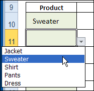
When you create a drop down list with data validation, you can’t change the font or font size. If you have reduced the zoom setting for a worksheet, it can be difficult to read the items in the list. And even at 100%, it can tough to read the tiny print, at the end of a long workday. Here’s how you can make data validation list appear larger.
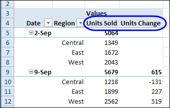
A pivot table is a great way to summarize data, and most of the time you probably use a Sum or Count function for the values. For example, in the pivot table shown below, the regional sales are totaled for each week. We can also use a built-in feature to calculate differences in a pivot table.
Do you use the free Pivot Power add-in that’s available on my Contextures website? I created Pivot Power to make my own work easier to do, and shared it on my website to help you with your pivot table tasks.
It automates some of the features that aren’t built in to an Excel pivot table, and makes some of the buried Excel pivot table features easier to access.
For example, there is a command that changes all the data fields to SUM, which is handy when Excel defaults to COUNT.
Get Free Pivot Power Add-In
Click here to go to the download page for this free add-in is still available, and try it out!
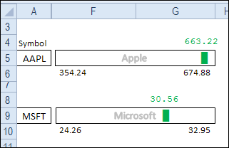
Today we’ll create an in-cell chart that shows the latest price for a stock, compared to its low and high prices. There is a sample file available for download, and a video that shows the steps.
If you’re using a named Excel table, you can apply a style that shades alternate rows with colour. In the table shown below, the row shading has two rows of grey followed by one row of white.
To create this table style, I duplicated one of the existing styles, and modified the row shading.
duplicate one of the existing Excel table styles
If you don’t want to use a table, or table styles aren’t available in your version of Excel, you can still have shaded rows, by using conditional formatting.
Shade Rows With Conditional Formatting
To shade the rows, we’ll use the MOD function in a conditional formatting formula. To see how it works, we can test the MOD function on the worksheet, in column G.
We want a set of 3 rows – two with shading, and then a row with no colour. With the MOD function, we’ll get the remainder, if the row number is divided by 3.
=MOD(ROW(),3)
The result for each row is shown in column G, and is either 0, 1 or 2.
We can shade rows where the result is 0 or 1, and leave the rows with 2 as no fill colour. To check the result of the MOD function, we can add a formula in column H, to see if it’s less than 2.
=G2<2
If the result is TRUE, we can shade the row. I’ve highlighted the TRUE cells in the screen shot above, to show which rows will be shaded.
Columns G and H were just used to test the formula, so I’ll clear those out, before formatting the cells.
Create a Conditional Formatting Formula
To shade the rows, we’ll combine the MOD function and the test of the results, in a conditional formatting formula.
Select the cells where you want the banded rows to appear. In this example, cells A2:F9 are selected.
On the Ribbon’s Home tab, click Conditional Formatting, then click New Rule
For Rule Type, click on Use a Formula to Determine Which Cells to Format
For the formula, enter =MOD(ROW(),3)<2
Click the Format button.
On the Patterns tab, select a colour for shading – light grey was used in this example
Click OK, click OK
The selected range has two rows of grey shading, followed by a row with no fill colour.
Make the Shaded Rows Adjustable
In the previous example, the numbers 3 and 2 were typed into the conditional formatting formula. To make the shading adjustable, you could enter the numbers on the worksheet, and then refer to those cells in the formula.
On the worksheet, create an input range for the numbers. In this example, the numbers are entered in J1 and J2, and the sum of those numbers is in J3.
Modify the Formula
To change the conditional formatting formula:
Select a cell in the range where the conditional formatting rule was applied. In this example, cells A2:F9 are selected.
On the Ribbon’s Home tab, click Conditional Formatting, then click Manage Rules
Click on the MOD rule in the list of rules, and click Edit Rule
Change the formula, so it refers to the grey shading number — $J$1, and the total number — $J$3:
=MOD(ROW(),$J$3)<$J$1
Click OK, click OK
Test the Shading
To test the interactive shading formula, change one or both of the numbers in J1:J2. The shading on the worksheet should automatically adjust.
In the screen shot below, the numbers were changed so there is one grey row, followed by 2 rows with no fill.
Watch the Video
To see the steps for creating shaded rows on the worksheet, please watch this short video tutorial.
Download the Sample File
To download the sample file, please visit the Conditional Formatting Examples page on my Contextures website. The Excel 2010 / 2007 sample file contains the interactive example.
______________________________
If you want to scroll down the worksheet, and lock the heading rows in place, so they’re always visible, you can use the Freeze Panes command. Be careful though, or you might end up with hidden rows that you can’t get to.
As I show in the video, to alternate between functions, such as SUM, AVERAGE or MAX in a summary row, use the Subtotal function in your formulas.
Then, add a drop down list of functions on the worksheet, using the Excel data validation feature. Next, select the function you want, to see those results in the summary.
This technique does not require macros — the formulas create the changing summaries.
Do you ever get sent an Excel file, and asked to figure out why it’s not working correctly? The odds are that it was created several years ago, by someone who has left the company, and a few other people have “improved” it over the years.
Now it’s a mess, and nobody is sure exactly how it works. It’s up to you to sort it out. Lucky you!
Here’s how I start the troubleshooting process, and you can see the steps in the video below. There are detailed instructions on my Contextures site.
Make a Copy of the Original File
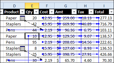
In the screen shot below, you can see a worksheet that is similar to the ones that I troubleshoot. There is a rainbow of colours on the sheet, but they don’t seem to have any significance – they’re just someone’s favourite colours.
I’ll get rid of that rainbow, and colour the cells that contain:
formulas
text
numbers
data validation
But the first step is to make a copy (or two) of the original file, and store it in a safe place. Don’t make any changes to the file, until you have that backup file safely stored away – you might want to refer to it later, as you dig deeper into the troubleshooting.
Price Calculation Sheet with coloured cells
Clear All Colour
The next step is to remove all the colour fill from the worksheet, so you can add your own colour scheme.
Select all the cells on the worksheet
Choose No Fill as the cell fill colour
When you’re finished troubleshooting, and the worksheet is functioning correctly, you can clear the troubleshooting formats.
Then, add colour to the data entry cells, or other key cells, to help people understand how the workbook should be used.
Colour the Formula Cells
The next step is to find and format the cells that contain formulas.
On the Ribbon’s Home tab, click the Find & Select command
Click on Formulas, to select all the formula cells
Then, use the Fill command on the Ribbon to format the Formula cells. I usually use grey for the formula cells, which indicates that they shouldn’t be changed.
Colour Remaining Cells
Next, you can find and format the cells that contain constants, and data validation, by using the other options in the Find & Select drop down.
On the Ribbon’s Home tab, click the Find & Select command
Click on Constants, then format the Constant cells.
Repeat the steps to format the Data Validation cells, where drop down lists or special rules apply
Colour Constant Numbers
Finally, find and format the cells that contain constant numbers. These might be data entry cells, that you can use in testing the worksheet.
On the Ribbon’s Home tab, click the Find & Select command
Click the Go To Special command.
Select Constants, and check the box for Numbers. Remove the check mark in the Text, Logicals and Errors boxes, then click OK.
Then, format the constant number cells
Finish Worksheet Formatting
After all the key cells are colour coded, you can add a legend on the worksheet, to show what the colours mean.
Then, get started with the troubleshooting. For example, in the screen shot below, the circled cells contain constants, but they should contain formulas.
get started with worksheet troubleshooting
Watch the Formatting Video
To see the steps for formatting the different types of cells, you can watch this short video.