
Recently, I enrolled in an online Infographics and data visualization course, and the classes started last week. In one of my homework assignments, I used this trick to link pivot chart title to report filter.
Allow Other Entries With Excel Drop Down List
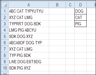
To make data entry easier, add a drop down list on an Excel worksheet. That way, people can choose from the list, instead of typing a product name. If you want to allow other entries with Excel drop down list, follow the steps below, to enable that option.
Continue reading “Allow Other Entries With Excel Drop Down List”
Excel INDEX MATCH Lookup Formula
Recently, my daughter, Sarah, broke her foot, and has had two surgeries, with orthopaedic specialists trying to put all the pieces back together.
I stayed with her for a few days after the latest surgery, to help her out.
One night, just as I was dozing off, I got a message on my iPhone. It was my daughter, texting from the next room.
- “Are you still awake?”
- “Yes, what do you need?”
- “I need help with Excel.”
That made me laugh, and I went in to see what help she needed.
Event Planning with Excel
Sarah is the event planner at Movember Canada, and is organizing launch parties for this year’s Movember events, across Canada.
“During November each year, Movember is responsible for the sprouting of moustaches on thousands of men’s faces, in Canada and around the world. With their “Mo’s”, these men raise vital funds and awareness for men’s health, specifically prostate cancer and male mental health initiatives.”
Of course, event planning is more difficult when you’re confined to your bed, but she’s been going non-stop, despite her injuries.
Apparently the surgical staff had to pry the phone from her hand in the last seconds before she was wheeled into the operating room. Now that’s job dedication!
Excel List of Invitees
Sarah had a list of invitees to the Movember events, and was trying to match email addresses with a short list of people who had not responded to their invitations.
The short list did not include the city name, and she wanted to pull that data from the original list.
Here, using some fake data that I created, is an example of the Excel worksheet, with the long list, and short list.

Solving Problem With Index and Match
Like many other Excel problems, this one can be solved with a combination INDEX/MATCH formula.
- The MATCH function finds the email in the original list, based on an exact match
- The INDEX function pulls the City from that email address’ row.
INDEX/MATCH Formula
In cell J4, I entered the following formula:
=INDEX($D$4:$D$1000,MATCH(I4,$E$4:$E$1000,0))
The formula looks for the city in column D, in the row where the matching email address was found in column E.
Copy Formula Down
Next, I copied the formula down to the last row in the short list, and all the cities showed up in the short list.

Finally, I copied the City cells in the short list, and pasted them as values, because the formulas weren’t needed any more.
Back to Sleep
It only took a couple of minutes to fix my daughter’s Excel problem, and she thanked me for coming to the rescue.
It warms a mother’s heart to know that her children grew up to be productive adults, who use Excel every day. Sarah might not remember that formula later, but that will give her a reason to call me the next time that she’s stuck in Excel.
After helping out, I headed back to the guest room, and fell asleep. I’m not sure how much longer Sarah kept working, but probably way too long.
And if you’re growing a moustache in support of Movember, please let me know!

_____________________
Create Excel Line Column Chart on 2 Axes
When you create a chart in Excel 2010, you can select one of the chart types on the Ribbon’s Insert tab. Microsoft Excel won’t let you select two chart types at the same time though.

Restrict Date Entries with Data Validation
With Excel’s data validation, you can restrict the dates that can be entered on a worksheet. For example, you could specify start and end dates on the worksheet, and only dates within that range can be entered.
Start and End Dates on Excel Sheet
In the screen shot below, start and end dates are entered in column E, and dates in column B must be within that date range.

Set Up the Data Validation
After entering the start and end dates on the worksheet, follow these steps to set up the data validation:
- Select the cells where the data validation will be applied – cells B2:B6 in this example.
- On the Excel Ribbon, click the Data tab, and click Data Validation
- From the Allow drop down, select Date
- From the Data drop down, select Between
- Click in the Start Date box, and click cell E1, where the Start Date is entered.
- Press the F4 key, to change the cell reference to an absolute reference — $E$1
- Click in the End Date box, and click cell E2, where the End Date is entered.
- Press the F4 key, to change the cell reference to an absolute reference — $E$2
- Click OK, to close the Data Validation window.

Watch the Video
To see the steps for applying this data validation, please watch this short video tutorial.
It also shows you how to set up a formula that will validate dates from today, to 6 days from now.
More Date Validation
Here’s another example of data validation for dates in Excel. This video shows 3 ways to validate dates.
- Specify a starting date and an ending date. (Date option)
- Show a drop down list of valid dates (List option)
- Create a rule in a custom formula (Custom option)
Written instructions, and the sample file, are on the Data Validation for Dates page, on my Contextures site.
______________________
Excel Error 1004 When Pasting Filtered Data
It should have been a simple task in Excel VBA – copy a filtered range, and paste it into a new workbook. How many times have you written code to do that, and it always runs without problems?
However, last week a client sent me a file where that simple code wasn’t working. While copying and pasting the filtered range, an error message kept popping up:
Run-time error ‘1004’: Paste method of Worksheet class failed.

Look For the Obvious Problems
I figured there was some simple and obvious reason for the error, and went through the code, looking for problems.
I tweaked a few lines in the code, where there were ambiguous references, but nothing helped. That annoying error message kept popping up. And, ,to add to the confusion, the data had been copied onto the worksheet, despite the error message.
A Google search was fruitless – there were many people complaining about similar problems, but no solutions that appeared to work. At least there weren’t any solutions that I could find.
Most of the suggestions were to change the order of the steps, because Excel might be losing the copied data, before it could paste. I tried that too, and it didn’t change anything.
External Ranges in the Filtered Data
Finally, I noticed that there were External Data ranges in the sheet where the filtered data was located. It seemed unlikely, but maybe those ranges were interfering with the copy and paste. So, I deleted those names, and tried the macro again. Amazingly, it worked!
I added code to delete those ranges as part of the macro, in case more External Data ranges are added to the data in the future.
Code to Delete Named External Ranges
In my client’s workbook, all the external data range names started with “ExternalData_”, so I used that to find the ranges and delete the names.
Here is the bit of code that I added to the top of the macro.
Dim nm As Name
For Each nm In ThisWorkbook.Names
    If InStr(nm.Name, "ExternalData_") > 0 Then
        nm.Delete
    End If
Next nm
The Problem Comes Back
Unfortunately, after running the revised macro for a while, the error message came back, even though the external data ranges had been deleted.
Maybe there were new ranges, that had different names, or perhaps deleting the external data ranges was just a temporary fix.
My client added an “On Error Resume Next” line to the macro, to get past the problem section, and that’s working fine for now.
As a better solution, I suggested using an Advanced Filter to extract the data to the new workbook, because is very fast (except in Excel 2007), and doesn’t create the same error message.
You can record a macro as you manually run an Advanced filter and then tweak the code to make it flexible. See the steps and a video in this blog post: Advanced Filter Macro
Still a Problem in Excel 2010
The workbook that my client sent was created in Excel 2003, and that’s were I did the testing, and found the solution.
To see if the problem was fixed in newer versions of Excel, I tested the workbook in Excel 2007 and Excel 2010. If the External Data ranges were not deleted, the same error message appears when you run the copy and paste code.
So, if you run into this error message, and none of the obvious solutions help, check for External Data, and delete those ranges, if possible. If you use this solution, please let me know if it works permanently, temporarily, or not at all.
__________________________
Spreadsheet Day 2012
Do you have your party plans finalized? Remember, tomorrow, October 17th, is Spreadsheet Day, in honour of the date that VisiCalc was first shipped.
Last year, the theme was spreadsheets for students, and I posted a student time tracker in which you can plan your projects and track your class and lab hours.
![]()
In 2010, I posted my top 5 Excel tips, that I had seen posted on Excel blogs over the previous year. One of those tips was Jon Peltier’s tutorial on making vertical bullet graphs.

Top 5 Excel Tips for 2012
This year, I’m going back to the top 5 theme. Every week, in my Excel News email, I link to interesting articles that I’ve found on other blogs. Some are simple tips, others are more complicated, and some are food for thought.
Below, in no particular order, are my favourites from those articles. And if you’re not on my Excel News mailing list, please add your name, by using the form at the top right.
VBA Conditional Formatting of Charts by Value and Label
Jon Peltier, who creates time-saving Excel chart utilities, shared his technique for building charts with conditional formatting that is based on the values and labels.
In the screen shot below, the Beta bar is dark red, because its value is high, and the Alpha bar is very light blue, because its value is low.

Force Clients to Enable Macros
If you’re creating automated workbooks for other people to use, you might run into problems if those people don’t click the button to enable the macros. That macro warning can be easy to overlook, or it might not even appear, if security level is set to High.
[Bacon Bits blog is no longer online]
Mike Alexander, in his Bacon Bits blog, explains how he solves the problem, by Forcing Your Clients to Enable Macros. Users can’t miss the giant message in his workbooks, and they can’t do any work until they enable macros.

Who Says the Ribbon Is Hard?
Bob Phillips convinces us that it’s easy to make dynamic changes to the Excel Ribbon. In his article, Bob explains how to use Excel VBA to change the Ribbon commands.
He shares his sample code, and you can click the link to download his sample workbook. The link opens as an Excel Web App, so click the File tab, then click Download a Copy, to save a copy on your computer.
Create an Interactive Sales Chart
Chandoo posts hundreds of great Excel tips on his blog, so it was hard to pick just one for this list of favourites. However, I finally selected this interactive sales chart example, because it incorporates several useful techniques.

You can use Chandoo’s example to build your own dashboard with a dazzling interactive chart. Download the sample file, and poke around in the code, to see how it works.
Microsoft Excel Check List Template
On his Clearly and Simply blog, Robert Mundigl has created an Excel template for a structured Checklist. It gives you the option to check and uncheck by double clicking.
That’s a feature that many people like, so you can use download the Microsoft Excel Check List Template and use the same technique in your workbooks.

What Are Your Favourite Excel Tips?
It was tough to pick a top 5 Excel tips, and I’m sure there are many other tips that you found. If you have favourite articles from the past year, please share a link in the comments below.
____________
Find Text With INDEX and MATCH
Is there a harder working team in Excel, than the reliable duo of INDEX and MATCH? These functions work beautifully together, with MATCH identifying the location of an item, and INDEX pulling the results out from the murky depths of data. See how to find text with INDEX and MATCH.
Make All Queries Replicable in Access
Recently, I’ve been making changes to an Access database that someone else built. In most cases, that’s enough of a challenge, but this database has an extra hurdle – it’s set up for replication.
Access Database Design Master
One copy of the database is set up as a Design Master, and replicas are made from that copy. Everyone can make changes and additions in their copy, then all the copies are synchronized, to pull all the data together.
I hit a snag, right near the end of the development phase, so I’m posting this solution, in case it helps someone else — or me, later, when I need the code again. 😉
Don’t Move the Design Master
I’ll spare you the gory details, but all the structural changes have to be made in the Design Master. If that file is lost or corrupted, you can create a new Design Master from one of the replicas in the set.
My client sent me the Design Master to work on, and I’ve been busily making changes for several weeks. Now, it’s time to send it back, so they can use all the fancy new forms and reports.
Unfortunately, I learned that when the Design Master is moved from its original folder (i.e. when the client sent me a zipped copy), the moved copy becomes a replica.
Create a New Design Master
So, I had to get another copy of the database, with all the current data, and strip out everything except the tables. Then, I imported all the queries, forms and reports from the new version, and will send it back to my client.
When they get the database, they’ll make it the Design Master, and create new replicas for everyone to use.
It’s an annoying workaround, but we’ve done a few tests, and it works fine.
Make the Queries Replicable
It’s easy to do an import of all the forms, queries and reports that are in another database, and that step took just a couple of minutes. However, all the imported objects should come in marked as “Replicable”, because that is property setting in the other database.
The forms and reports were fine, but none of the queries had the Replicable property turned on. There are over 100 queries, and I wanted a way to turn on that property programmatically, not manually.
You’d think that would be easy, but I spend a long time searching in Google, Bing, and my shelf full of Access books. Nothing helpful appeared in the search results, but I didn’t give up!
Finally, I found an article, written in 1999, on the Microsoft website, and it had the code I was looking for — Implementing Database Replication with JRO
Set a Reference
The code has to run from another database, so I used a different copy of the client’s database. The database with the queries to update is closed.
In the database where I put the replication code, I had to set a reference to JRO in the Visual Basic Editor (Tools > Reference)

The Replication Code
The following code will change Replicable setting for the specified object to True.
Sub MakeObjectReplicable(strDBPath As String, _
                         strObjectName As String, _
                         strObjectType As String)
   Dim repMaster      As New JRO.Replica
   repMaster.ActiveConnection = strDBPath
   repMaster.SetObjectReplicability strObjectName, strObjectType, True
   Set repMaster = Nothing
End Sub
Loop Through the Queries
The sample code in the article only changed one query, but I wanted to change them all. The database I used to run this code had all the same queries as the target database, so I looped through its queries.
As you can see in the code comments, even though I’m updating queries, the object type is “Tables”. I tried “Queries” first, but that didn’t work, and then I noticed this warning in the Microsoft article:
Important Even though the SetObjectReplicability property provides an ObjectType argument to specify the type of object you are working with, the argument only accepts a value of “Tables” for both queries and tables.
The code runs quickly, and this will be handy if we ever have to rebuild the Design Master. Use this at your own risk though – I’m certainly not a Replication expert, and it might not work in all cases.
Sub MakeAllQueriesReplicable()
Dim strPath As String
Dim strFile As String
Dim qry As QueryDef
strPath = "C:\Data"
strFile = "MyNewDesignMaster.mdb"
on error resume next
For Each qry In CurrentDb.QueryDefs
	'NOTE: object type 'Tables' is used for both tables and queries
	MakeObjectReplicable strPath & "\" & strFile, qry.Name, "Tables"
Next qry
End Sub
____________________________
Midnight Times Missing in Excel Worksheet
Last week, I was working on a client’s time sheet file, and noticed something strange. The worksheet was used to record shift start and end times, and I was testing the calculations, to make sure that everything was working correctly.
Time Past Midnight
Shifts that run past midnight can cause problems, so I tested that scenario, and I also tested shifts that started at midnight. I wanted to be sure that everyone would get all the pay they were entitled to!
In column D, I calculated the hours worked, by subtracting the start time from the end time, and adding 1 to the end time, if it was in the next day. Here is the formula in cell D2:
=(C2+IF(OR(C2=0,C2<B2),1,0)-B2)*24

Missing Midnight
The calculations were working well, but the cells where I had entered a midnight time appeared empty.
Fortunately, the calculations still worked, even with the missing start times.
I know that midnight is a favourite time for mysterious things to happen in horror movies, but was my worksheet haunted? Was this an early Halloween prank?

Hidden Zeros
Finally, I realized that someone had formatted the worksheet to hide the zeros. And, if your worksheet is formatted to hide zeros, the midnight times won’t show, because they are equal to zero – 0:00
To fix the problem, I turned the Show Zeros setting back on, and all the midnight times came out of hiding.
To show zeros on a worksheet
Here are the steps I followed, to show the worksheet zeros:
- At the top left of the Excel window, click the File tab, then click Options.
- At the left, click the Advanced category
- Then, scroll down, and in the Display options for this worksheet, add a check mark to “Show a zero in cells that have zero value”
- Click OK to close the Options window.

Unhide Your Zeros
I had forgotten all about this problem, until someone left a comment on my blog yesterday, asking why the midnight times weren’t showing in her worksheet.
At least I’m not the only one who has had this mysterious problem, and if it has happened to you, I hope this tip helps.
It’s not one of Excel’s most complicated problems, but it’s the little things that can drive you crazy. 😉
____________________________