While working on a project, such as creating a database, or programming an Excel file, I make notes about the changes I’m making.
Before quitting for the day, I add a few notes on what steps should be taken next. For example, “Create a data entry form” or “Add project codes list”.
This makes it easier to get up and running the next time I resume work on the project.
If you use this technique, you won’t have to spend several minutes reviewing your work to figure out where you left off — your “Next Steps” notes will jog your memory. Well, most of the time!
Did you know that it only takes one keystroke to create a chart from data in Excel? Here are the simple steps to create a very quick Excel chart.
First, select a cell that contains the chart data, or select a heading in one of the data rows or columns
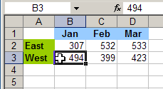
In the screen shot below, the data is in A1:D3, and cell B3 is selected.
NOTE: Cell A1, at the top left corner of the chart data is empty. That makes it easier for Excel to create a quick chart.
Next, on the keyboard, press the F11 key
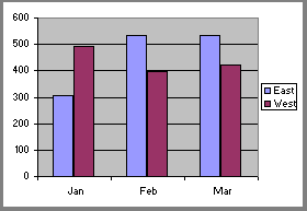
A chart sheet is inserted in the active workbook, with a chart in the default chart type, as shown below.
In the sample workbook, the default chart type is a Clustered Column. There are two columns for each month, with East in light purple, and West in dart purple..
Just remember — this is a super quick way to add a chart in Excel. After you insert that Excel chart so quickly, don’t be tempted to spend another couple of hours playing with the formatting, to make it look perfect!
If you use an Excel command frequently, or if an Excel command isn’t available on the Excel Ribbon, you can add its icon to the Quick Access Toolbar (QAT).
Throughout the day, I log in to several web sites that require a user name and password. I store them all in a list in an Excel workbook, but it’s tough to remember all of them, and easy to waste time guessing.
A couple of months ago a colleague recommended RoboForm, so I downloaded the trial version. (Thanks to Ross Connell.)
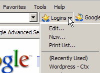
Life became much easier! A RoboForm toolbar appears at the top of my web browser, and I can select a Login from a drop down list. That takes me to the selected site and enters the user name and password.
If I go to a new site and enter a user name and password, RoboForm automatically asks if I’d like to save the new Login.
When the trial period ended, I bought the RoboForm Pro version, and at $29.95 US, it’s been well worth the price. No more time wasted in fumbling for passwords. For home use, you could continue to use the free version, which limits the number of Logins you can store.
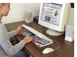
If you waste time searching for pens, paper clips and other small office items, a keyboard with storage space might save you time.
These are available for purchase on-line, from the Keyboardorganizer.com web site. They come in plain white or black, with stock artwork, or your own custom design.
As you work on your computer, you probably open several applications, and the Windows Taskbar quickly fills with buttons.
The buttons you need most might be stuck at the far right, or in a hidden row of buttons, and that can slow you down.
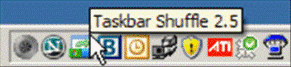
Taskbar Shuffle is an easy-to-use free utility that gives you control over the taskbar button placement. You can download the utility, and read more details, at the FreeWebs website.
When installed, Taskbar Shuffle appears as an icon in the System Tray:
Another handy feature of the Taskbar Shuffle is the ability to rearrange the icons in the System Tray.
Move the icons you use most so they’re at the left, closest to your mouse pointer, and it’s easier to click on them when you need them.
While working on an Excel 2003 worksheet, you might want to colour a few of the cells, change the font colour for the text, or add borders to a range of cells.
Select a Fill Colour
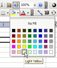
To add colour, you select a cell, click on the drop-down arrow at the right side of the colour button on the toolbar, and click on a colour.
This process is simple enough, but all those trips up and down from the toolbar can get a bit tiring, and take extra time.
Select Fill Colour
To Save Time, Move the Palettes
If you have lots of formatting to do, it will be easier if the palettes are closer to the area where you’re working.
You can detach the palettes from the toolbar, and move them onto the worksheet.
Note: This feature is not available in Excel 2007, or later versions.
Move Excel Palette
To move one of the “tear away” palettes (Font Color, Fill Color, or Borders), follow these steps:
On the toolbar, click the drop-down arrow, to open the palette.
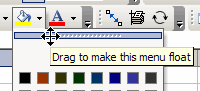
At the top of the palette, point to the thin grey bar.
When your pointer changes to a four-headed arrow, drag the palette down onto the worksheet.
Open a Floating Palette
Close a Floating Palette
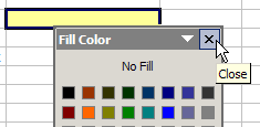
When you’ve finished working with the palette, click the X at its top right, to close it.
Close a Floating Palette
Video: Move Excel Toolbar Colour Palettes
And here’s a short video, if you’d like to see the steps for moving one of the Excel 2003 palettes.