Create Alternating Shaded Rows on Excel Sheet

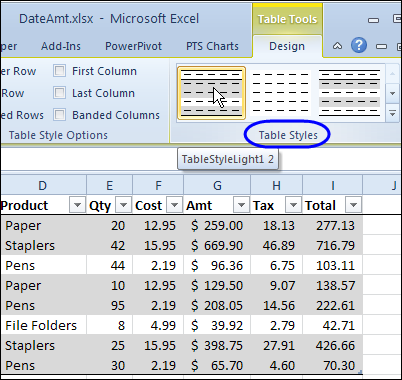
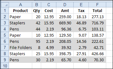
If you’re using a named Excel table, you can apply a style that shades alternate rows with colour. In the table shown below, the row shading has two rows of grey followed by one row of white.

To create this table style, I duplicated one of the existing styles, and modified the row shading.

If you don’t want to use a table, or table styles aren’t available in your version of Excel, you can still have shaded rows, by using conditional formatting.

Shade Rows With Conditional Formatting

To shade the rows, we’ll use the MOD function in a conditional formatting formula. To see how it works, we can test the MOD function on the worksheet, in column G.

We want a set of 3 rows – two with shading, and then a row with no colour. With the MOD function, we’ll get the remainder, if the row number is divided by 3.

=MOD(ROW(),3)

The result for each row is shown in column G, and is either 0, 1 or 2.

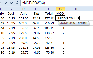
We can shade rows where the result is 0 or 1, and leave the rows with 2 as no fill colour. To check the result of the MOD function, we can add a formula in column H, to see if it’s less than 2.

=G2<2

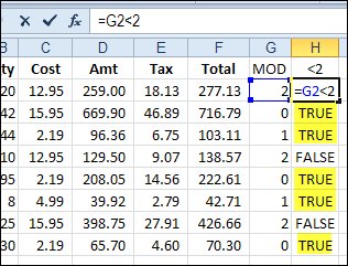
If the result is TRUE, we can shade the row. I’ve highlighted the TRUE cells in the screen shot above, to show which rows will be shaded.

Columns G and H were just used to test the formula, so I’ll clear those out, before formatting the cells.

Create a Conditional Formatting Formula

To shade the rows, we’ll combine the MOD function and the test of the results, in a conditional formatting formula.

1. Select the cells where you want the banded rows to appear. In this example, cells A2:F9 are selected.
2. On the Ribbon’s Home tab, click Conditional Formatting, then click New Rule
3. For Rule Type, click on Use a Formula to Determine Which Cells to Format
4. For the formula, enter =MOD(ROW(),3)<2
5. Click the Format button.
6. On the Patterns tab, select a colour for shading – light grey was used in this example
7. Click OK, click OK

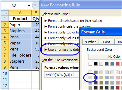
The selected range has two rows of grey shading, followed by a row with no fill colour.

Make the Shaded Rows Adjustable

In the previous example, the numbers 3 and 2 were typed into the conditional formatting formula. To make the shading adjustable, you could enter the numbers on the worksheet, and then refer to those cells in the formula.

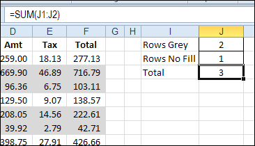
On the worksheet, create an input range for the numbers. In this example, the numbers are entered in J1 and J2, and the sum of those numbers is in J3.

Modify the Formula

To change the conditional formatting formula:

1. Select a cell in the range where the conditional formatting rule was applied. In this example, cells A2:F9 are selected.
2. On the Ribbon’s Home tab, click Conditional Formatting, then click Manage Rules
3. Click on the MOD rule in the list of rules, and click Edit Rule
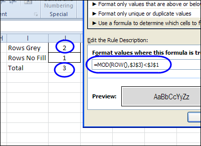
4. Change the formula, so it refers to the grey shading number — $J$1, and the total number — $J$3:
   • =MOD(ROW(),$J$3)<$J$1
5. Click OK, click OK

Test the Shading

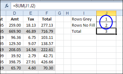
To test the interactive shading formula, change one or both of the numbers in J1:J2. The shading on the worksheet should automatically adjust.

In the screen shot below, the numbers were changed so there is one grey row, followed by 2 rows with no fill.

Watch the Video

To see the steps for creating shaded rows on the worksheet, please watch this short video tutorial.

Download the Sample File

To download the sample file, please visit the Conditional Formatting Examples page on my Contextures website. The Excel 2010 / 2007 sample file contains the interactive example.
______________________________