There is a new function in Excel 2013 – FORMULATEXT – that lets you show the text from a cell’s formula.
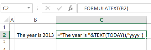
In the screen shot below, cell C2 contains the formula:
=FORMULATEXT(B2)
cell C2 contains FORMULATEXT formula
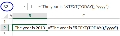
Matches Formula Bar
The FORMULATEXT result shows the formula that’s in cell B2, just as if you had clicked on cell B2 and looked in the formula bar.
Use FORMULATEXT for Troubleshooting
You can use FORMULATEXT for auditing or troubleshooting a worksheet. For example, combine FORMULATEXT with the INDIRECT function, to check the formula in any cell.
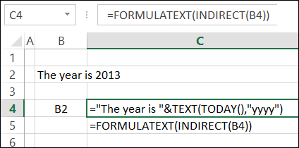
In the screenshot below, a cell address (B2) is entered in cell B4, and the FORMULATEXT result shows the formula from cell B2.
=FORMULATEXT(INDIRECT(B4))
FORMULATEXT result shows the formula from cell B2
More on FORMULATEXT
For more FORMULATEXT information and examples, please visit my Contextures website. You can read the details there, and download the sample file: Excel FORMULATEXT Function
Video: Excel FORMULATEXT Function
To see the steps for creating a FORMULATEXT function, and a few examples, you can watch this short video tutorial.
Yes, I know that it’s a bad idea to use the SendKeys method in Excel, because strange things can happen.
However, it’s handy in a few situations, and I use SendKeys in a few of my Comments macros.
SendKeys Example
For example, in this macro to insert a blank comment, without a user name, the comment opens for editing, at the end of the macro.
Sub CommentAddOrEdit()
Dim cmt As Comment
Set cmt = ActiveCell.Comment
If cmt Is Nothing Then
ActiveCell.AddComment text:=""
End If
SendKeys "+{F2}"
End Sub
Send Keyboard Shortcuts
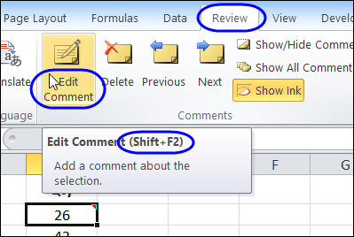
In that example, the SendKeys line simulates using the keyboard shortcut – Shift + F2 – to edit the comment in the active cell.
Shortcut keys to edit comment Shift + F2
SendKeys Doesn’t Run
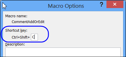
While I was updating the Comments VBA page, I wanted to test a few of the macros, to make sure that they still worked in Excel 2010. To make it easier to run a macro, I added a keyboard shortcut for it – Ctrl + Shift + C.
Macro Options Shortcut Key setting
Shortcut Problem
When I tested the macro, using that shortcut, it inserted the comment, but the comment didn’t open for editing. Hmmm…maybe that shortcut code doesn’t work in Excel 2010.
But, when I ran the macro from the Macro window, instead of the shortcut, it worked correctly. So, the problem wasn’t the SendKeys code.
There was something funny happening with the shortcut to run the macro.
The problem occurs because this is a very short macro, and I was still pressing the Ctrl + Shift keys when the macro runs the SendKeys statement. And that messes up the SendKeys keystrokes. See – I told you that SendKeys was risky!
Suggested Solution
The suggested solution is to add a Wait line in the macro, just before the SendKeys code. So, I altered the macro, and now it runs correctly when I use the keyboard shortcut.
Sub CommentAddOrEdit()
Dim cmt As Comment
Set cmt = ActiveCell.Comment
If cmt Is Nothing Then
ActiveCell.AddComment Text:=""
End If
Application.Wait (Now() + TimeValue("00:00:01"))
SendKeys "+{F2}"
End Sub
Last week, you saw how to open and edit the Ribbon code in an Excel file that has a custom tab. This week, you can see how to create a custom tab in an Excel workbook, and add buttons to run your macros.
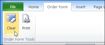
This example is based on an Order Form workbook, and the buttons run macros to clear the data entry cells, and to view the file before printing.
You’ll see how to set the custom tab labels and icons, and change your macros so they run from a click on the Ribbon. Exciting, right?
Watch the Video
To see the steps, please watch this video. It’s a bit longer than the videos that I usually make, but the steps are quite easy, so give it a try!
Download the Sample File
To see the written instructions, and to download the sample file, please visit my Contextures website: Add Custom Ribbon Tab to Workbook
Excel Dashboard Course Re-opens
Custom ribbon tabs can make your workbooks easier to use, and they add a professional touch. If your goal is to build a dashboard, Mynda Treacy from My Online training Hub is opening her Excel Dashboard Course, and if you sign up by January 30th, you can get it for 20% off.
The course is video based, delivered online and is available 24/7. You also receive comprehensive workbooks and sample dashboards to keep. There’s even an option to download the videos.
The previous classes were very successful, and you can read the glowing reviews from the students, who loved all the techniques that they learned in the course, and are using them to impress their colleagues.
Click here to find out details of the course, read the student comments, and watch the ‘behind the scenes’ video that shows you what you’ll receive as a member.
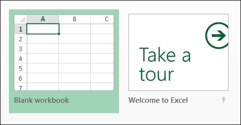
If you’ve been using Excel 2013, you might enjoy seeing the collection of templates when you open Excel. There is a blank template at the top left, and you can even take a tour of Excel.
Have you created any custom tabs for your Excel files? I avoided that, as long as possible, but have finally started dabbling with the Ribbon code.
And, the good news is that it’s not as dark and scary as I imagined.
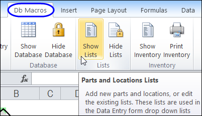
Here is a screen shot of a sample file that I created, as an update to my Parts Database which has a UserForm for data entry.
When the file opens, it adds a custom tab to the Ribbon, with buttons to run the workbook’s macros.
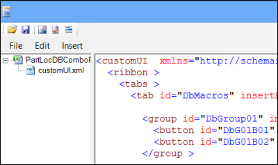
To see the Ribbon code, without messing with the hidden parts of an Excel file, you can use the free tool – Custom UI Editor. (UPDATE: No longer available)
To get started, use the Custom UI Editor to take a look at a sample file or two. Then, you can copy some of the sample code into your own files, and tweak the labels and macro names, to match your workbook.
Watch the Video
To see the steps for opening and editing the Ribbon code with the Custom UI Editor, you can watch this short video. The sample file and written instructions are here: Excel Ribbon Custom Tabs Intro
You know that it’s time to update a web page, when all of the dates in the examples are 2002. Apparently, I’ve been creating Excel sample files for a long time!
Happy New Year! I took a couple of weeks off, and I hope that you had some time to relax too. Now, it’s a new year, and time to get back to work.
It’s tough work staring at your computer all day, so maybe you’ve decided to set a couple of health goals for 2013. I’m getting out for a walk every morning, which is a great way to start the day. It’s good exercise, and all that fresh air helps my brain get going too!
If you’re looking for help with keeping track of calories, or weight loss, you can download a couple of free files from my Contextures website, to make things easier.
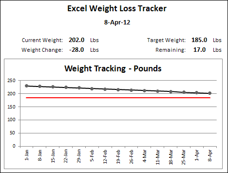
For weight tracking, try my Weight Loss Tracker. You can choose either pounds or kilos as the weight measurement, and enter your targets and daily data.
There is also a version for Stone and pounds, if you prefer that system.
Who knew that this would still be a problem in Excel 2013? Almost 4 years ago, I posted about numbers not lining up, when Excel was zoomed to less than 80%
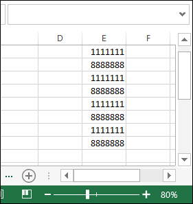
Now I’m working on a new laptop, and realized that the problem is back. In Excel 2013, I’m using the default font – Calibri 11. Here’s a list of numbers, at 80% zoom.
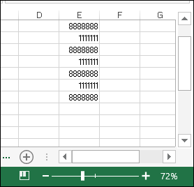
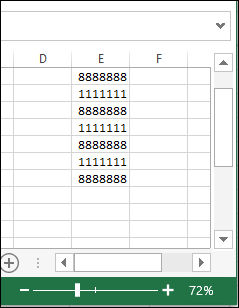
And here is the same list at 72% zoom – the numbers have changed to a proportional font, and the 1111111s are much narrower than the 8888888s.
Change the Registry
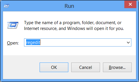
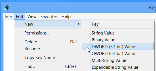
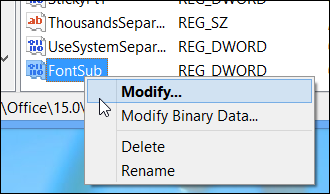
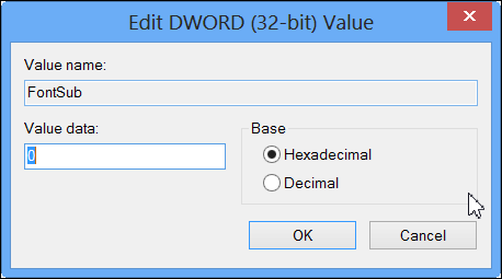
To fix the problem, I followed the instructions that I posted in April 2009, when I was setting up my previous laptop. Here they are again, with adjustments for Windows 8 and Office 2013. The original instructions came from this MSKB article:
In the old days, if you opened a file that contained macros, a warning message popped up on the screen. That has changed, and now Excel 2010 runs macros without enabling, in some situations.