Change All Pivot Charts With One Filter

Slicers were introduced in Excel 2010, and they make it easy to change multiple pivot tables with a single click.

Note: In earlier versions, you can use programming to change the report filters in multiples pivot tables.

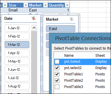
AlexJ has shared a space-saving technique for using a single Report Filter to update multiple pivot tables. This technique uses slicers, but they are stored on a different worksheet, so they don’t take up room on the dashboard.

Single Report Filter

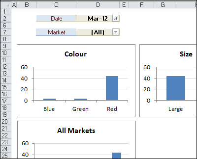
Here is a screen shot of AlexJ’s dashboard, with two filters at the top of the sheet. The pivot charts are all connected to the same Date slicer, so when you select a date, all the charts change.

Multiple Filters

You can use more than one filter with this technique, and I’ve added a Market filter too. The third chart is not connected to the Market filter – it always shows the results for all markets.

Note – If you’re using more than one master filter, AlexJ warns us to leave a few blank rows between them. Otherwise, you’ll see a message that pivot tables can’t overlap one another.

Show Details Feature

Just remember that there is a problem with the Show Details feature, when you use slicers.

If you don’t have the slicer fields in the pivot tables, you might see all the data, instead of the filtered data, when you double-click on a value cell.

With this technique though, the pivot tables are stored on a separate sheet, which could be hidden from the users, so that reduces the problem.

Watch the Video

To see the steps for creating the pivot charts, and connecting them through a slicer, watch this short video.

Download the Sample File

To see how AlexJ’s technique works, you can visit my Contextures website, and download the sample file. On the Sample Excel Files page, go to the Pivot Tables section, and look for PT0031 – Change All Pivot Charts With One Filter.

The technique will work in Excel 2010, and later versions, where slicers are available.

____________________