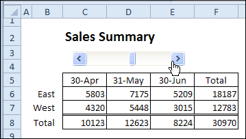
If you’re building Excel reports for other people to use, you can add a few interactive chart features, to let people customize the reports.
In this example, there is a check box beside each region name, in the sales summary table.
Excel tips and tutorials

If you’re building Excel reports for other people to use, you can add a few interactive chart features, to let people customize the reports.
In this example, there is a check box beside each region name, in the sales summary table.
A couple of months ago, I shared an example with a scroll bar that selects the dates for an Excel report. There is a pivot table on a hidden sheet, and a summary report uses GetPivotData formulas to pull data from that pivot table.
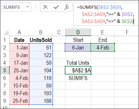
First, some news about the upcoming Office 365 launch, and then a tip on how to sum for a date range in Excel.
When you’re setting up data validation on a worksheet, you can include an Input Message, to help anyone who’s using the workbook.

You’ll have to get to the point quickly though – the message is limited to 255 characters.
There are other limitations too – you can’t control the size of the text box, and you can’t change its font size or fill colour, unless you change your Windows settings.
As an alternative to the Input Message popup, you can show a message in a text box, at the top of the worksheet. In the text box, you can set the font type, font size, font colour, and fill colour, to suit your worksheet.

The Input Message display is turned off, but the Title and Message are entered in the data validation window.

There is a sample file on my website that you can download, and instructions for this technique on my Contextures website: Display Input Messages in a Text Box
The original sample file uses the input message text, which is limited to 255 characters. In an email, Richard G. asked about showing a longer message in the text box.
So, I’ve created a new sample file, that uses most of the code from the original example, and adds a new feature. Now, you can create a list of Input Message Titles, and the message that you want to display for those titles.

Then, when you click on a data validation cell, its title is used as a lookup in the messages table. If there is an entry for that title, the Additional Message text is added to the end of any existing Input Message text. Then, the entire text string is shown in the text box at the top of the worksheet.

To download either the original sample workbook, or the Longer Message sample file, please visit my Contextures website: Display Input Messages in a Text Box
The files are zipped, and they contain macros, so remember to enable macros when testing the files.
___________________
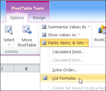
A few months ago, I shared my code for listing all the formulas in an Excel workbook. The code creates a new worksheet, with details on each formula’s worksheet name, cell address, the formula and the formula in R1C1 format.
If you’ve been following the Canadian news (and who isn’t?), you know that the penny has been eliminated from circulation. To honour the occasion, Google made a special doodle for google.ca on February 4, 2013.

If you’re shopping with cash now, the final amount will be rounded up or down, to the nearest nickel. There are guidelines posted on the Royal Canadian Mint’s website: Eliminating the Penny: Rounding [article no longer available]

As an example, the Mint’s website shows the purchase of coffee and a sandwich, with tax, for a grand total of $4.86.
The tax department says to round the tax to the nearest cent, so you can use Excel’s ROUND function for to calculate the HST. Just multiply the subtotal by the tax rate, and round to 2 decimal places. Here is the formula in cell B6:
=ROUND(B5*D6,2)

With the HST, the grand total for the lunch is $4.86. We don’t have pennies now, so the cash payment will be rounded to the nearest nickel. Excel’s ROUND function can’t help with that.
Fortunately, there is another rounding function – MROUND – that can round to a specified amount.
In this example, we want to round the grand total, which is in cell B7. We’ll enter the multiple in cell B9, to show how the cash payment was rounded.
Here is the cash payment rounding formula in cell B10:
=MROUND($B$7,$B$9)

A nickel is worth 5 cents, so what happens if you enter a 5 in cell B9, to use as the multiple?

Oops! That rounds the amount to 5 dollars, instead of the nearest nickel.
Change the amount in cell B9 to 0.05, which is the way that you’d enter a nickel amount in a worksheet.

Perfect! With the MROUND function, and a multiple of 0.05, you can round those sales totals to the nearest nickel.
____________________

________________
There is a sample file on my Contextures site, in which you can enter invoice details, then print all the new invoices by clicking a button.

I’ve updated the file, and you can now download the xlsm version, if you’re using Excel 2007 or a later version.
In the new version, the invoice data is stored in a named Excel table, and a named range – Database – is based on that table. The range is dynamic, because it is based on the named table, so it will include new rows as they are added.
Invoices that have been printed are marked with an X, and the new invoices do not have a mark in column A.

On the Invoice sheet, you can see how many invoices have not been printed. A formula calculates that number by counting invoice numbers and subtracting the count of X marks:
=COUNTA(Data!B2:B25)-COUNTA(Data!A2:A25)

When you click the Print Invoices button, a macro filters the list, to show only the records with a blank cell in column A. This code is quite different from the previous version, because it uses List AutoFilter VBA, which is only available in newer versions of Excel.
Then, for each of those records, the invoice is printed, and then the record is marked with an “X”.

To see how the invoice printing macro works, and to view the code, you can download the sample file. On the Sample Spreadsheets page, go to the Functions section, and look for FN0009 – Print Unmarked Invoices
The zipped file is in Excel 2007/2010 format (xlsm), and contains macros.
___________________
If you’d like a quick and easy way to add dates in a worksheet, you can use this handy date picker tool, from Jim Cone.
The Date Picker opens to the current date, and you can scroll through months and years, by using the scrollbars at the top of the date picker form.

Just select a cell, and click the insert button, to add the date. If you hold the Shift key, and click the Insert button, it will append the date to the cell’s contents.

In addition to inserting the date, Jim’s date picker will also add a calendar to the worksheet – either a single month, or a full year.

To see all the details, and to download the date picker file, please visit my Contextures website: Excel Date Picker
The file is in Excel 2003 format, and contains macros, so enable macros if you want to test the file. The VBA code is unlocked, so you’ll be able to poke around in the code, and see how it works.
Jim hasn’t tested the file in Excel 2013, but a quick test in that version worked fine for me.
__________________
Last week, we took a look at the new FORMULATEXT function in Excel 2013. Another one of the new features in Excel 2013 is the ISFORMULA function.
Finally, there’s a way to identify cells that contain a formula, without creating a User Defined Function to do the job.

The TYPE function was originally designed to show what a cell contained, such as text or a formula. It returns a number to show the type for a cell’s contents, or a formula’s result.
Here’s the list of results, and the data types:

In a few versions of Excel, the Help files incorrectly reported that a formula would return 8 with the TYPE function, but unfortunately, that’s not the case.
With the new ISFORMULA function, you can test a cell, to see if it contains a formula.
In the screenshot below, the following formula is entered in cell B4, and copied across to cell D4:

The result in cells B4 and C4 is FALSE, because cells B2 and C2 have numbers typed in them.
The result in D4 is TRUE, because cell D2 contains a formula.
You can use the ISFORMULA function with conditional formatting, to highlight cells that contain formulas.
In the screen shot below, cells in column C have a formula, and they are shaded grey.

For the details on how to apply this type of conditional formatting, and for more information on the ISFORMULA function, you can visit my Contextures website: Excel ISFORMULA FUNCTION
_____________________
There is a new function in Excel 2013 – FORMULATEXT – that lets you show the text from a cell’s formula.
In the screen shot below, cell C2 contains the formula:
=FORMULATEXT(B2)

The FORMULATEXT result shows the formula that’s in cell B2, just as if you had clicked on cell B2 and looked in the formula bar.

You can use FORMULATEXT for auditing or troubleshooting a worksheet. For example, combine FORMULATEXT with the INDIRECT function, to check the formula in any cell.
In the screenshot below, a cell address (B2) is entered in cell B4, and the FORMULATEXT result shows the formula from cell B2.
=FORMULATEXT(INDIRECT(B4))

For more FORMULATEXT information and examples, please visit my Contextures website. You can read the details there, and download the sample file: Excel FORMULATEXT Function
To see the steps for creating a FORMULATEXT function, and a few examples, you can watch this short video tutorial.
______________