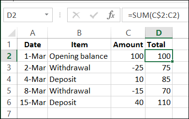
If you’re using a pivot table, there are built in features that lets you show a running total, or a percent running total. Here’s the command to show a % Running Total in a pivot table.
Continue reading “Create a Running Total in an Excel Column”
Excel tips and tutorials

If you’re using a pivot table, there are built in features that lets you show a running total, or a percent running total. Here’s the command to show a % Running Total in a pivot table.
Continue reading “Create a Running Total in an Excel Column”
With Excel’s conditional formatting, you can highlight cells based on specific rules. There are some built-in rules available, and you can use formulas to create your own formatting rules.
To see the steps for setting up the conditional formatting, watch this short video. The written steps are below the video.
To download the sample file, go to my Contextures website: Highlight Duplicate Records in a List
In this example, we want highlight duplicate records in a table. There is a built-in rule for highlighting duplicate values in a single column, but nothing that will check an entire row.
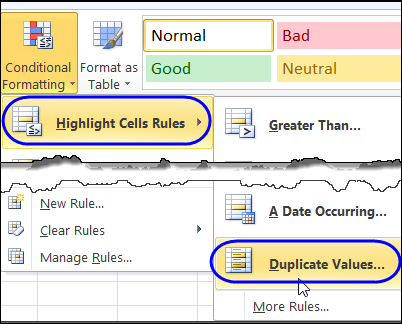
So, we’ll create our own rule, and it will require a new column on the worksheet, before we add the conditional formatting.
In the sample data, there are two identical rows, and these should be highlighted after we apply our conditional formatting.
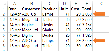
The first step is to use the CONCATENATE function to combine all the data into one cell in each row.
Add a new heading in cell G1 – AllData – and in cell G2, enter this formula, to combine the data from all the cells in that row.
=CONCATENATE(A2,B2,C2,D2,E2,F2)
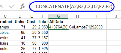
Next, copy the formula down to the last row of data.
Then, a conditional formatting rule is set, to color the rows that are duplicate records. We’ll use the COUNTIF function to check for duplicates in the AllData column.
=COUNTIF($G$2:$G$8,$G2)>1
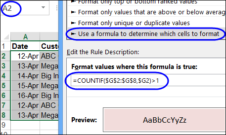
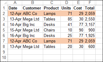
If there is more than one instance of a data combination, that indicates a duplicate row, and the cells in columns A:F will be coloured. The two rows with duplicate records are highlighted, so our conditional formatting formula worked!
For detailed instructions, and to download the sample file, go to my Contextures website: Highlight Duplicate Records in a List
_________________________
When you create a list in Excel, do you automatically convert that list to a formatted table?
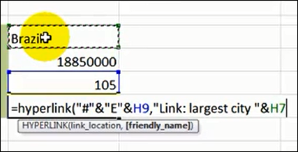
Last week, I heard from Kevin Lehrbass, who runs the My Spreadsheet Lab website. Kevin has posted an Excel video on YouTube, that shows how you can make a dynamic hyperlink, using array formulas.
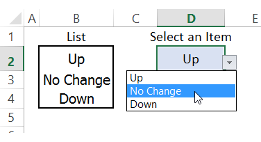
To make data entry easier, you can create a drop down list in an Excel cell, using data validation.
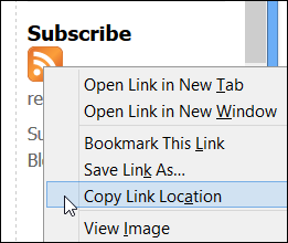
As you’ve heard, Google Reader will be disappearing in a few months <sigh>, and we’ll have to find other ways to follow our favourite blogs. I’m looking for a replacement, but haven’t found anything perfect yet. How about you?
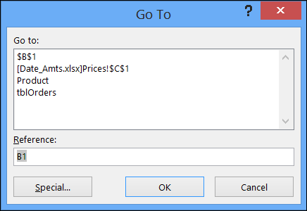
In Excel, you can create named ranges, and go to those ranges by selecting a name from the Name Box.
Yesterday, one of my clients emailed to let me know that she was having trouble entering January dates in a file that I had created.
My first guess was that there was an issue with the regional settings, because her company uses the dd/mm/yyyy format.
But when I tried entering a January date, with my mm/dd/yyyy settings, I got an “Invalid date” message too.
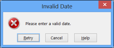
The date that I had entered – 1/3/13 – was a valid date and in a valid format, so I checked the data validation settings. And that’s where I found the problem.
The cell had been restricted to dates from 60 days prior to the current date:
=TODAY()-60
and up to 60 days after the current date:
=TODAY()+60
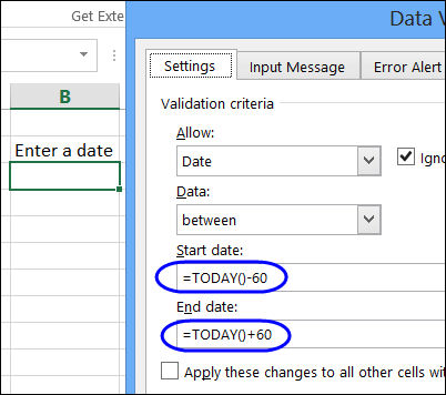
Those date range settings had made sense when we set up the file. The date range limits prevented people from accidentally entering strange dates, such as mistyping a year – 2031 instead of 2013, for example.
Do you ever find records like that in your database or workbook? It can really mess things up!
Anyway, a simple change to the data validation formula fixed the problem. Instead of 60 days, I changed the formulas to 120 days.
=TODAY()-120
and
=TODAY()+120
It still prevents those year typos, but gives my client a bigger window for entering data in the file.
In this video, three different data validation methods are used to validate dates. From the Allow drop down in the data validation settings, the following options will be used:
Video Timeline:
For more examples of data validation for dates, you can visit the Excel Data Validation – Dates page on my Contextures website.
_____________
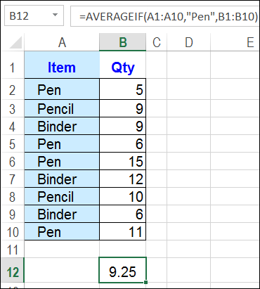
In Excel, you can use the SUMIF and COUNTIF functions, to sum and count values, based on criteria. Did you know that you can also calculate an Excel average, based on multiple criteria?
This week, Dick Kusleika posted his Amazon Linkerator – an Excel file lets you create links to Amazon products.
First, you find a product on Amazon, and copy its web page URL. Then, open the form, enter a product code and description, and it creates a link for you.
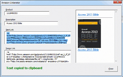
It’s very fancy, and you can download the sample file, to try it for yourself. It uses an Excel UserForm, and you can modify the code to add your own information.
Jimmy Pena has an Amazon Link Builder too, and you can see the details here: Amazon Link Builder
I build Amazon links too, and you can see lots of them on my Excel Book List page.
To create my links, I use worksheet formulas, instead of a fancy UserForm. If you like things simple, you can try this method.
You enter the product code and product title, and then copy the link or the HTML code, and paste it into your blog post or web page.
WARNING: Check the latest information on the Amazon website, to be sure that these short links are still permitted. Their policies can change at any time.
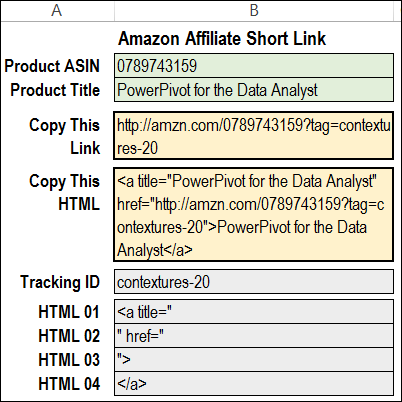
First, a link is created in cell B5, from the Amazon URL, the product code (ASIN) and the Tracking ID.
=https://amzn.com/ & ProdCode & “?tag=” &TrackID
Note: Cell B3 is formatted as Text, because some codes start with a zero, and you don’t want Excel to remove those.
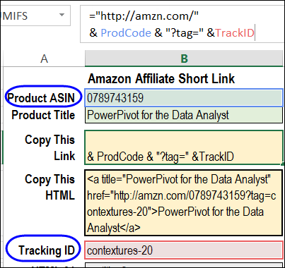
Then, that link is used in the to create the HTML code in cell B7.
The four HTML cells have snippets of text that are required for building the HTML code. The formula in cell B7 combines the product title and the link, with four snippets of text.
=HTML_01 & ProdTitle & HTML_02 & ProdLink
& HTML_03 & ProdTitle & HTML_04
To test the Amazon link formulas, you can download my sample file, from the Excel Sample Files page on my Contextures website. In the Functions section, look for FN0025 – Build Amazon Affiliate Links
____________________