Last week, I heard from Kevin Lehrbass, who runs the My Spreadsheet Lab website. Kevin has posted an Excel video on YouTube, that shows how you can make a dynamic hyperlink, using array formulas.
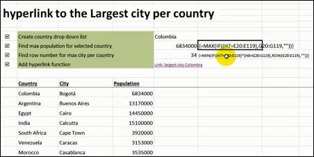
Select a country from a drop down list, and click on the hyperlink to go to the selected country’s largest city. Well, you’ll go to that location in the table – you won’t actually end up in the city!
Select a Country
At the top of the worksheet, Kevin created a drop down list of countries, by using data validation. You’ll start by selecting a city in that cell.

Find the Largest Population
In the cells below the city, Kevin uses array formulas to find the largest population for that country, and the row in which that population is found.

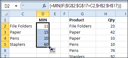
If you need help with this step, you can see the instructions for MIN IF and MAX IF on my website, and watch my short video. It uses an example with office supply quantities.

Create a Hyperlink
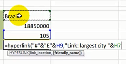
Next, Kevin creates a hyperlink formula that uses the row number and city name. The # sign at the start of the reference is how you link to a cell within the workbook.
Click on the link to go to the selected country’s largest city. Of course, you’ll go to that location in the table – you won’t actually end up in the city.

You can find more details on the HYPERLINK formula, and another short video, on my Contextures site: Excel HYPERLINK Function
Watch the Video
To see how to create the dynamic hyperlink, watch Kevin’s video. At the end of the video, Kevin combines the separate formulas into one large formula. You could skip that step, if you’d rather, and just hide rows 8 and 9, with the population and row formulas.
______________

Very interesting!
I made a similar blog post a few months ago about how to locate lookup values in a table [HYPERLINK].
Love this idea! Here are a couple of ideas I had for extending this:
1. Add a rank column as the first column of data (this will make calculations simpler)
2. Use the DMIN to find the lowest rank that matches that country. (No need for array functions)
3. Use Index to look up the largest city and population based on the rank returned
4. Link to the entire matching table row, instead of just the population cell
5. Add in some conditional formatting to highlight either the matching row, or all rows that match the selected country.
6. Fix the Hyperlink cell style so the link stays blue
7. Add a conditional hyperlink to the left of the data to return to the top of the worksheet [=IF(selRank=$B9,HYPERLINK(“#A1″,5),””) A 5 in Webdings is an up arrow]
Here is the mockup Dynamic Hyperlinks
The drop down for country will not show on the Excel Web App, so please download the file to gain the full functionality.
You can also dynamically expand the table rather than hard code the range