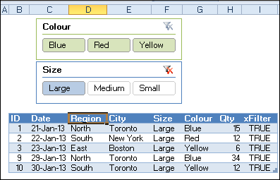
Pivot table filtering was improved in Excel 2010, when Slicers were introduced. Instead of using the drop down lists in the pivot table headings, you can click on a Slicer, to quickly filter the pivot table. You couldn’t use Slicers to filter a table in Excel 2010 though.
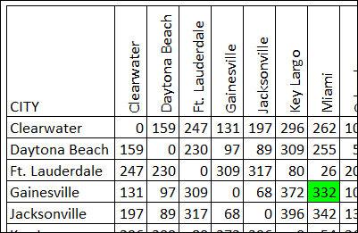
There is a new sample file on my website, in response to a lookup question that someone asked on my Contextures Facebook page. The sample file shows how to get mileage from Excel lookup table, when you pick two cities.
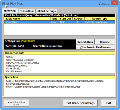
A few years ago, Ron Coderre created his PivotPlay PLUS Add-in that you can download from my Contextures site. This free add-in was designed for Excel 2003, and lets you view and edit the connection strings for pivot tables and query tables that are based on external data queries.
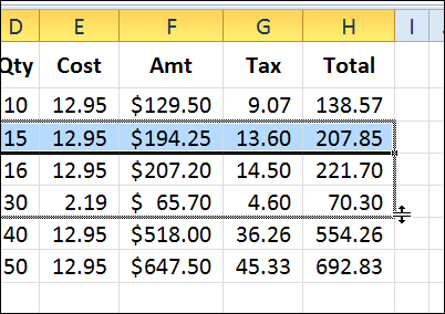
If you want to insert a block of cells on a worksheet, what method do you use most often? Do you insert rows with Excel fill handle, or with a command?
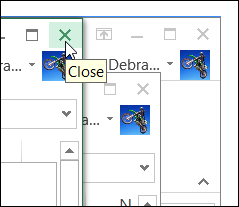
One of the new features in Excel 2013 is that each file opens in a separate window. Having each file in its own window makes it easier to compare files side-by-side, and most of the time I like the separate windows.
It’s been a bad week for Excel, with big news stories about spreadsheet errors. Two Harvard professors were in the news after a student at the University of Massachusetts found errors in their economic research paper.
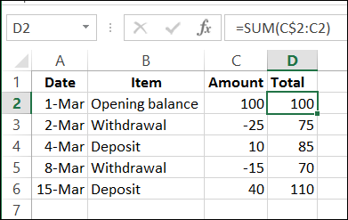
If you’re using a pivot table, there are built in features that lets you show a running total, or a percent running total. Here’s the command to show a % Running Total in a pivot table.
To see the steps for setting up the conditional formatting, watch this short video. The written steps are below the video.
To download the sample file, go to my Contextures website: Highlight Duplicate Records in a List
Highlight Duplicates
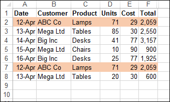
In this example, we want highlight duplicate records in a table. There is a built-in rule for highlighting duplicate values in a single column, but nothing that will check an entire row.
built-in rule for highlighting duplicate values
So, we’ll create our own rule, and it will require a new column on the worksheet, before we add the conditional formatting.
Concatenate the Data
In the sample data, there are two identical rows, and these should be highlighted after we apply our conditional formatting.
two identical rows in sample data
The first step is to use the CONCATENATE function to combine all the data into one cell in each row.
Add a new heading in cell G1 – AllData – and in cell G2, enter this formula, to combine the data from all the cells in that row.
=CONCATENATE(A2,B2,C2,D2,E2,F2)
formula to combine the data
Next, copy the formula down to the last row of data.
Apply the Conditional Formatting
Then, a conditional formatting rule is set, to color the rows that are duplicate records. We’ll use the COUNTIF function to check for duplicates in the AllData column.
=COUNTIF($G$2:$G$8,$G2)>1
create new conditional formatting rule
If there is more than one instance of a data combination, that indicates a duplicate row, and the cells in columns A:F will be coloured. The two rows with duplicate records are highlighted, so our conditional formatting formula worked!