Excel Conditional Formatting Update

The holidays are a great time to catch up on tasks. I’ve updated another popular Excel video — Colour a Row Based on a Cell Value in Excel.

To continue the conditional formatting theme, here are a few articles that you might have missed, when they were originally posted.

Watch the Conditional Formatting Video

Watch this short video to see how to colour a row based on a cell value in Excel.

There is a full transcript following the video.

Video Transcript:

With Excel’s conditional formatting, you can easily highlight a cell if it’s over or under a certain value, or if it meets a value that you’ve set.

But in some cases, instead of just a single cell, you might like to highlight a whole row in a table, if one of the cells in that row is over a certain number or under.

In this case, we would like to highlight each row in this list if the number of units sold is greater than 75.

So to do that, I’m going to select all of the rows, all of the columns in each row. So I’ve selected from A2 down to D10.

On the Ribbon, on the Home tab, I’ll click Conditional Formatting, and none of these preset rules will do exactly what I want. So I’m going down to New Rule, and in here I’ll select a formula.

So I’m going to use a formula to determine how to color each row.

When I click that, there’s a spot where I can put the formula.

I want to, in each row, look at the value that’s in column B. So I’ll type =

And we want, from every column, we want to look at column B. So we have to lock that cell. We don’t want it to be relative, we want it to be absolute.

So type a $ to lock that in. And then B.

And we want, in this case, the active cell we can see is white, where the other cells are highlighted with blue.

We can see that, in the name box, A2 is showing up. So that’s the active cell, so the active row is 2. So I’m going to type 2 here.

We’re going to check what’s in B2 and see if it’s greater than 75. So that’s our test.

And if it is greater than 75, we want to format it. So I’ll click Format and I’ll choose a fill color, maybe a blue color and click OK, and click OK again.

And now, any row where the number of units is greater than 75, all four cells in that row are colored blue.

______________
Excel Data Validation Update

I’ve finally updated my Data Validation intro video, so it shows the steps for creating a drop down list in Excel 2010, instead of Excel 2003.

Note: These instructions apply to Excel 2007 too, in case you’re using that version.

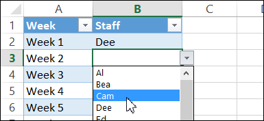
Data Validation Drop-Down List

Data Validation Articles

In honour of this momentous occasion, here are links to a few of my previous Excel Data Validation articles and posts.

You probably know all the basics, but maybe you’ve missed a few of these tips and tricks.

Show or Hide User Tips In Excel – AlexJ shows how to let users turn data validation messages on or off, by choosing TRUE or FALSE from a drop down list.

Dependent Data Validation From a Sorted List – Select an item in the first drop down list, and related items are shown in the second drop down list.

Limit the Total Amount Entered in Excel – use Data Validation to limit the total amount that users enter in a group of cells.

Select Multiple Items from Excel Data Validation List – instead of selecting just one item from a data validation drop down, you can select two or more.

Plan Your Party Seating with Excel – too late for Christmas dinner, but this might help with your New Year’s festivities.

Note: Remember to vote for the Excel functions that you’d like to learn more about during the 30 Excel Functions in 30 Days challenge, starting January 2nd.

Watch the Excel Drop Down List Video

The shiny new video is below, in case you’d like to see the steps for making a drop down list in an Excel worksheet.

________________

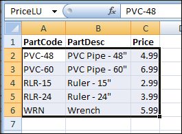
Combine Values for Excel VLOOKUP

Do vampires prefer a specific blood type? Type A? Type B? Type AB? Are you positive? During the holidays, they might drink glögg, or Cosmopolitans!

Anyway, Marsha probably isn’t a vampire, but she wants to choose A or AB when doing a VLOOKUP. Here’s how you can combine values for Excel VLOOKUP formulas.

Continue reading “Combine Values for Excel VLOOKUP”

2011 Challenge: 30 Excel Functions in 30 Days

Icon30Day Your great suggestions in the Improve Your Excel Skills comments got me thinking. What skills would I like to improve in 2011?

It’s hard to pick just one thing, but I’ll start with Excel functions. Even the functions that you use every day can have hidden talents, and pitfalls that you aren’t aware of. And there are so many functions, that you probably only use a fraction of them.

So, in January, let’s explore 30 Excel functions in 30 days. Yes, you’re right — there are 31 days in January. However, I’m being kind, and will give you the first day off, to recover from your hangover, and/or post-holiday exhaustion. 😉

CHOOSE Your Functions

For this challenge, we’ll stick to functions in the Text, Information and Lookup and Reference functions, listed below.

There are about 60 functions in the list, and we can only cover 30, so please vote for your favourites. If you can’t see the list below, click here to go to the form.

Deadline for voting is Wednesday, December 29, 2010, at 5 PM (Toronto time).

Share Your INFO

We’ll start the challenge on January 2nd, and go till January 31st. Please check the blog every day during the challenge, and add your tips and comments, or even a HYPERLINK. There’s no SUBSTITUTE for team work, to ensure we ADDRESS all AREAS of each function.

My mind ISBLANK now, and I can’t FIND any more puns, so I’ll sign off now, and let you CHOOSE your functions. Thanks!

Update: Thanks for voting before the December 29th deadline — votes are no longer being accepted.
___________

Use Excel Scroll Bar to Trim Christmas Tree

An Excel scroll bar can be used for practical (and sometimes boring) things, like testing the effect of price changes, or adjusting a chart’s date range.

But this is the festive season, so let’s use a scroll bar for something more, well, festive!

Trim the Tree

In this example, instead of accounting and finance, you’ll see how to use an Excel scroll bar to decorate a Christmas tree, without macros.

Unfortunately, this Excel file can’t make hot chocolate or eggnog, so you’ll need to provide your own.

Useful Excel Features

It’s not just for the holiday season though — the sample file has useful features that you can adapt to other workbooks too:

  • Scroll bar lets users change a number quickly and easily
  • A text box that displays a changing message based on VLOOKUP formula
  • conditional formatting shows hidden cells when target number is reached
  • named ranges make it easy to work with specific cells
Use Excel Scroll Bar to Trim Christmas Tree

Watch the Video

To see how the Excel Christmas tree trimming scroll bar works, you can watch this short Excel video.

Excel Scroll Bar Sample File and Instructions

For instructions on creating the Excel scroll bar file, and to download the sample file, go to my Contextures website: Excel Scroll Bar Christmas Tree Example.

Improve Your Microsoft Excel Skills

Someone emailed me this week, and asked how he could improve his Excel skills.

Here’s what I suggested:

Books: Read Excel books – there’s a list of my favourites on my Contextures site, and you can browse your local bookstore, or search in Amazon, to see what’s new

Blogs: Follow a few Excel blogs, to see what topics people are writing about. You might learn about new Excel features, or see helpful tips for familial features

Websites: Visit some of the Excel expert websites, for Excel tips, tricks, videos, and sample files. I highly recommend the Contextures website, but I might be biased. 😉

Videos: Another great way to improve your Excel skills is by watching videos. There are lots of videos on my Contextures site, and on my Contextures YouTube channel.

Experiment: And remember keep trying new things in your own Excel files! That’s my favourite way to learn. Just be sure to do your tests on a backup copy of your files, just in case things go horribly wrong!

Your Suggestions

What would you add to that list of ways to improve your Excel skills?

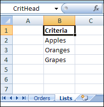
Excel AutoFilter With Criteria in a Range

In Excel 2003, and earlier versions, an AutoFilter allows only two criteria for each column. In Excel 2007 and later, you can select multiple criteria from each column in the table. See how to apply an Excel AutoFilter with  multiple criteria in a range on the worksheet.

Update: Get the latest version of this workbook on my Contextures site: Filter Criteria List Macro.

Continue reading “Excel AutoFilter With Criteria in a Range”

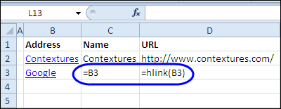
Get the URL from an Excel Hyperlink

Last week on the Bacon Bits blog, Mike Alexander showed how to send an email with the HYPERLINK function in Excel, complete with subject line and message.

Mike’s article showed how versatile the HYPERLINK function can be, and you also learned about Mike’s unique talent for poetry.

In the steps below, I’ll show you how to get the URL from an Excel Hyperlink.

Continue reading “Get the URL from an Excel Hyperlink”

Excel 2007 AutoFilter Dynamic Dates

icondynamic Over on the Contextures website, I’ve updated the AutoFilter Intro page, so it now covers the basics for Excel 2007 AutoFilters.
However, many people are still using an older version of Excel, so I’ve moved the original material to the Excel 2003 AutoFilter Basics page.

Improvements in AutoFilters

AutoFilters are easier to use in Excel 2007 and Excel 2010, and the filter and sort options are automatically added in the top row, if you format your list as an Excel Table.

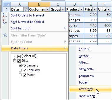
Filter for Dynamic Date Ranges

Among the new AutoFilter features that were introduced in Excel 2007 are dynamic date ranges.

A Dynamic Date Range is one that changes automatically, as time moves forward.

For example, you could select Yesterday, which will represent a different date, every day that you open the Excel file.

AutoFilter Dynamic Date Range settings

Update Filters

Unfortunately, the dynamic dates are only semi-dynamic, and they don’t magically change when you open the workbook at a later date. You’ll need to update the filter to see the current information.

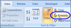
You can update the Excel 2007 AutoFilter manually, by clicking Reapply on the Excel Ribbon. Or, you could add a bit of code to the Workbook_Open event, to reapply the filters automatically.

autofilter2007_16

Learn More About Excel 2007 AutoFilters

If you’re not familiar with the new features in Excel 2007 and Excel 2010 AutoFilters, you can learn more at Excel 2007 AutoFilter Basics.
_____________