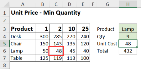
In some Excel workbooks, you might have a simple product pricing table, with the product name in one column, and the product price in the next column. With a simple VLOOKUP formula, you can get the price for any product.
In the video below, there’s a different kind of pricing table. There are product names in the first column, with quantity pricing information in the next four columns.
VLOOKUP and MATCH Formula
The VLOOKUP and MATCH formula in cell H5 finds the correct price for the selected product and quantity.
- =VLOOKUP(H3,A4:E7, MATCH(H4,A3:E3,1), FALSE)
Note: If your pricing lookup is in a Named Excel Table, see the video for a slightly different formula.
Video: Product Price based on Quantity
In this short video, you’ll see the steps for finding the product price, from the correct column, with VLOOKUP and MATCH.
Also, see a problem you might have with a named Excel Table, and how to change the formula, to solve that problem.
Video Timeline
- 00:00 Introduction
- 00:16 Product Prices
- 01:01 MATCH Function
- 02:32 VLOOKUP Formula
- 03:34 Excel Table
- 04:21 Fix the Formula
- 04:56 Get the Sample File
Get the Sample File
Get the sample file, and more VLOOKUP examples, from the VLOOKUP Function Examples page, on my Contextures website.
The zipped Excel file is in xlsx format, and does not contain any macros.
_____________________
Find Product Price Based on Quantity with Excel VLOOKUP and MATCH
_____________________


8 thoughts on “Find Product Price Based on Quantity with Excel VLOOKUP and MATCH”