
Last December, I posted an Excel Advent Calendar, and it was surprisingly popular, throughout the year.
Excel Advanced Filter Painfully Slow
Today, working on my Excel file was like riding a lazy snail through molasses in January — but slower!
Usually an Excel Advanced Filter is a speedy way to extract data from a table, but things weren’t working right in a sample file that I got last week.
And despite what my high school English teachers might think, you can’t mix too many similes, when trying to describe excruciating slowness.
Advanced Filter Macro Problem
The sample file had code that ran an Advanced Filter in Excel 2007.
The code ran quickly in Excel 2003, but screeched to a near halt in Excel 2007. What was the problem?
In the sections below, I detailed all the things I tried, while troubleshooting the slow macro problem.
- Tip: You can skip to the end, to see what the unexpected problem was, and how I finally fixed the Advanced Filter macro.
There’s a video at the end of this post too, where I show the problem and the solution.
The Slow Filter Symptoms
When the code ran in Excel 2007, it looked like the extracted rows were being pasted in the second worksheet, one row at a time.
Aha! I should turn off the screen updating — a simple solution. You’d think.
Nope! Even with the screen updating turned off, the code barely crawled along.
It took almost 3 minutes to extract 1500 rows — maybe a millisecond faster than it ran with screen updating turned on. Who has that kind of time?
Guess Again
In the next round of solution guessing, I got rid of the few formulas in the worksheet and criteria range.
There wasn’t anything too complex, but maybe that was slowing things down.
I also changed calculation to manual at the start of the code, then set it to automatic at the end of the code.
Neither of those changes had any effect on the code’s speed.
Strip the Data Clean
In round 12 of testing (I’ve lost track of the test count), I copied the data, and pasted it as values into a new workbook.
The code ran like lightning. In July. With jet engines. Hmmm.
Maybe it was the formatting and styles in the original file that were slowing things down.
To test that theory, I formatted the original table with Normal style, which removed all the borders and fill colour.
That didn’t improve things, but when I removed the red fill from the heading cells, I noticed a red comment marker in one of the cells.
Whip Things Into Shape
Could a comment be the problem? That didn’t seem likely, but:
- As soon as I deleted the comment, the code ran perfectly.
- When I put the comment back, the macro slowed to a crawl again.

Curiouser and Curiouser
When I tried to create a sample file to demonstrate this problem, things got even stranger.
I created a table with a comment in the heading, and ran the code, expecting it to be slow. It ran quickly, in several tests.

Add Shape to Worksheet
Next, I added a shape to the worksheet, and assigned a macro, to make it easier to run the code.
The code slowed down again!

Next, I deleted the shape, and the code was still slow, so I had to delete the comment to speed it up again.
The Verdict on Slow Advanced Filter Macro
If your Advanced Filters are running slowly in Excel 2007, try removing any comments in the table heading cells.
You could delete them at the start of a VBA procedure, run the filter, then add the comments at the end of the code.
Shapes + Comments = Trouble
The problem seems to occur if there are heading comments, and a shape is added later, as you can see in the short video demonstration below.
Fortunately, this problem appears to be fixed in Excel 2010, so if you upgrade, you should be able to have comments and shapes, without slowing down the Advanced Filters.
Another Solution
Update: In the comments, PDLobster suggests the following solution, to speed up the filters — thanks!
- Turn off all filters
- Select cell A1
- Turn Wrap Text ON
- Select the entire worksheet
- Turn Wrap Text OFF
Watch the Video
To see the steps for reproducing and solving the Advanced Filter speed problem, you can watch this short Excel video.
____________
Excel Copy and Paste Tips and Trouble
Copy and paste. It’s one of the first things you learn to do in Excel, and something you do every day.
Without copy and paste, your Excel work would take much longer, and you’d be exhausted by the end of the day, from all that typing!
Here are some Excel copy and paste tips and trouble shooting suggestions.
Continue reading “Excel Copy and Paste Tips and Trouble”
Holiday Preparations for Excel Overachievers
Last year, I posted a link to my Excel Christmas planner, that includes a scheduler for holiday meals.
Despite the rude comments from my Excel buddies (OCD? Torturing guests with pivot tables?), I still use that planner to stay on schedule.
Maybe those doubters go out for their holiday meals, so they don’t have to worry about planning!

Black Friday Sales Planner
Even if you don’t have to plan the holiday dinner, you might want to plan your Black Friday shopping trip, or compare gift prices at different stores.
In the latest version of the Excel Christmas Planner there’s a Black Friday worksheet.
Enter Store Names at the top of the table, then enter product info and prices in the rows below.

Find Best Prices
The worksheet calculates which store has the best price for each item, and which store has the most deals.
Note: If prices are the same at multiple stores, the first store will be shown in the “Best Price” column.

With this handy Excel Holiday Shopping worksheet, you’ll know where to start your shopping blitz, so you get the most for your money.
And that’s what the holidays are all about, right? 😉
Happy Thanksgiving!
__________
Automatically Change Excel Filter Heading
 There was a question about Excel Advanced Filter criteria on the Tech Republic blog recently, and I posted an answer.
A couple of weeks later, a Tech Republic mug and flag were delivered to my door, as a reward for answering.
It’s a Fragile Major Award
The real joy is in solving a problem, but it’s fun to get a major award, even if it’s not a fancy leg lamp that I can put in the front window.
Keep reading, to see what problem the blogger was having with Excel Advanced Filters, and download a workbook with my suggested solution.
Set Up an Advanced Filter
To use an Excel Advanced Filter, you create a criteria range, with headings that match the ones used in the original table.
Then, under one or more of the headings, you enter the filter criteria.
For example, in the screenshot below, the criteria would extract all the records where the quantity ordered is 20 and the product is juice.
With an Advanced Filter, you can even extract the data to a different location, all in one step.

Identical Headings
In most cases, when you set up an Advanced Filter criteria range, each heading must be identical to a heading in the source data table.
An easy way to make them identical is to link from the criteria headings to the table headings.
In the screenshot below, cell F1 has a formula with a link to cell B1.
- =B1

Different Headings
However, there’s one situation in which the criteria range headings must NOT match the table headings — if you use a formula in the criteria row.
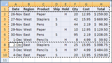
In the example below, we’d like to extract the records where the number ordered is different than the number shipped.
In the criteria range, there’s a formula in cell G2, to compare the quantity ordered and quantity shipped.
- =C2<>D2
Remove Criteria Heading
For this filter to work, the heading in cell G1 has to be removed, or changed to something different than any of the table headings.

Add a Space Character
Another option would be to leave the link to the table heading, and add a space character or underscore. That extra character makes the headings different
- =C1 & ” “

Create Adjustable Criteria Headings
This was the problem that the Tech Republic blogger encountered — remembering to manually change the heading, or remove it, when using a formula in the criteria range.
The question posed included this restriction:
Remember, you don’t want to force users to remember that in this particular case… they have to do something special like delete header text! Working with the list and criteria ranges, already in place, how would you get the desired results?
Heading With IF Formula
To make the heading adjust automatically, you can use an IF formula to test what’s in the cell below.
=C1 & IF(ISLOGICAL(G2), “_” , “” )
If cell G2 contains TRUE or FALSE, then it has a criteria formula, and an underscore is added to the heading.

Download the Advanced Filter Workbook
To see the data and the criteria range heading formulas, you can download the Advanced Filter Criteria Headings sample file. It’s in Excel 2003 format, and zipped.
The file contains a macro, that lets you run the advanced filter by clicking the Filter button on the worksheet. Enable macros if you want to use that feature.

Watch the Advanced Filter Criteria Video
To see the steps for applying an Advanced Filter, with regular criteria or a formula in the criteria range, please watch this short Excel video tutorial.
___________
Add Filter Markers in Excel Pivot Table
If you’re using Excel 2007 or Excel 2010, you can quickly see which fields in a pivot table have filters applied.
For example, in the screenshot below, the ItemSold field has been filtered.
The arrow drop down has changed to a filter symbol, with a tiny arrow.

Earlier Excel Versions
In Excel 2003 though, there’s no indicator that a field has been filtered. Here’s the same filtered pivot table in Excel 2003, and the drop down arrows look the same in both of the fields.
There’s no marker to show if either field has been filtered. You’d have to click each arrow, to see if any of the check marks have been removed from the pivot items. Who has time for that?

Create Your Own Filter Markers
Several of my clients are still using Excel 2003, and maybe you use it too. If so, you’ll appreciate this sample Excel file from AlexJ, which adds a bright blue marker above each filtered field.
That makes it easy to keep track of what’s been changed in the pivot table, and prevents you from overlooking the filters.
- Tip: You could even use these markers in newer versions of Excel. The bright blue arrows are easier to see than the tiny filter icons!

User Defined Function
To create the markers, Alex wrote a user defined function, named pvtFilterID.
In the screenshot below, you can see the pvtFilterID formula in cell D5, which refers to the ItemSold field heading in cell D7.
=pvtFilterID(D$7)
The formula is used in cells B5:D5, above the row fields, and that range could be adjusted if your pivot table has a different number of row fields.

The Blue Arrow Marker
Cell D1 is named Symbol.Filter, and it contains the blue arrow symbol that’s used as a marker.
If you changed the symbol there, the new symbol would be used as the filter marker.
In cell G5 there’s another formula, that shows a message if any of the pivot table fields are filtered.
- =IF(COUNTIF($B$5:$D$5,Symbol.Filter)>0, “Pivot Filter On” & Symbol.Filter,””)
This formula checks the cells above the pivot table, and shows the message if any of those cells contain the marker symbol.
Works With Slicers Too
Even though Alex wrote this code for Excel 2003 pivot tables, it works in Excel 2007 and Excel 2010 too.
In the screenshot below, you can see and Excel 2010 pivot table with slicers, and the filter markers highlight the row fields where filters have been applied.
The filter symbol is on the field drop downs too, and the bright blue markers are extra insurance that users notice which fields are filtered.

The Filter Marker Function Code
Here’s Alex’s code for the pvtFilterID function.
Function pvtFilterID(rng As Range) As String  'rng As Range)
On Error GoTo XIT ' -not in pivot
If Not rng.Parent Is ActiveSheet Then GoTo XIT
If rng.Cells.Count > 1 Then
    MsgBox "Error: pvtFilterID range selection"
    GoTo XIT
End If
If rng.PivotField.HiddenItems.Count > 0 Then
    pvtFilterID = [Symbol.Filter]
End If
XIT:
End Function
Clear the Pivot Table Filters
Another nice feature that was added to Excel 2007 pivot tables is the Clear All Filters command. Alex’s workbook contains a button that runs code to remove all the filters from a pivot table.
Here’s the code for the ClearPivotFilters procedure.
Sub ClearPivotFilters(ws As Worksheet)
    Dim pvt As PivotTable
    Dim pf As PivotField
    Dim pi As PivotItem
    Dim lSort As Long
On Error Resume Next
Set pvt = ws.PivotTables("PivotTable1")
For Each pf In pvt.VisibleFields
    If pf.HiddenItems.Count > 0 Then
      lSort = pf.AutoSortOrder
      pf.AutoSort xlManual, pf.SourceName
      For Each pi In pf.PivotItems
        pi.Visible = True
      Next pi
    End If
    pf.AutoSort lSort, pf.SourceName
Next pf
Set pi = Nothing
Set pf = Nothing
Set pvt = Nothing
End Sub
The button code passes the worksheet name to the procedure.
Private Sub cmdClearPvtFilters_Click()
    Call ClearPivotFilters(Me)
End Sub
Download the Sample File
To test the pivot table filter markers, and see the VBA code, you can download Alex’s sample file from the Contextures website.
On the AlexJ Sample Files page, go to the Pivot Tables section, and look for: PT0000 – Pivot Table Filter Markers
___________
Take a Break With Excel Games
It’s the middle of the week, and you’re buried under a pile of Excel workbooks. The weekend seems to be miles away.
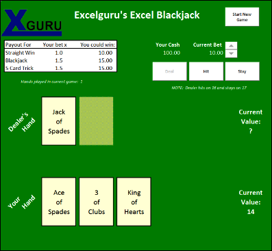
To get you over the midweek hump, here are three examples of spreadsheet fun and games.
Continue reading “Take a Break With Excel Games”
Show Us Your Spreadsheets
 Another humdrum day in the world of spreadsheets? Hardly!
Thanks to John Walkenbach (Mr. Spreadsheet) and Mike Alexander (DataPig), things are getting exciting.
They’ve just announced a Show Us Your Spreadsheets contest, with Excel books and gift cards going to the winners. The contest is open to residents of the USA, UK, and Canada (except Quebec).
How to Enter
To enter, send in a photo of yourself with one of John’s or Mike’s books, or with a fabulous Excel workbook that you created.
As an example of creative book holding, here’s John hiding behind a notebook, imitating the poses of his buddies Bill and Steve.

Read the Rules
Be sure to read and follow the official rules, and submit your photos (up to 3) by December 3rd.
You probably have some Excel books by John and/or Mike, but if not, head to Amazon or your local bookstore, and pick one up (or a bunch!)

Picking the Winners
The best photos will be selected by John and Mike, and prizes awarded based on their decision. These multi-talented gentlemen have previous experience in judging creative events, as you can see in the photo below.
Dick is constructing an amazing tower, and you can see John (second from left) and Mike (right), judging the event. This shows that they have a keen eye for design, and are calm in the face of danger.
They seem to like beer and hockey pucks too, so that bodes well for the Canadian entries!

____________
Get Date Year Month Day With Excel Functions
Sometimes, working with an Excel data import can be a rocky horror (text) show. This month, I’ve been working with a client who is pulling together data from several accounting systems.
The project is extra exciting because each system stores the data in a different format, and we have to assemble it into a common file.
I’m sure you’ve had to deal with a similar challenge, and used your mad scientist Excel skills to clean up the mess.
Imported Data – Date Formats
In one of the import files that my client uses, the date is stored in a YYYYMMDD format.
From that number, we have to calculate the transaction date, so Excel can understand it.
You can use a few Excel functions to extract the year, month and day, and turn that time warp into a valid date.
To quote the “Time Warp” song lyrics:
- It’s just a jump to the LEFT
- And then a step to the RIGHT
- Put your hands on your MID (hips)
Get Year with LEFT Function
In the screen shot below, the imported date is in column A. The year is at the left, in the first four characters.
Use the Excel LEFT function to pull those 4 digits into column C, to show the year.
- =LEFT(A2,4)

Get Day with RIGHT Function
The transaction day is shown in the two characters at the right of the date in column A.
Use the Excel RIGHT function to pull those two digits into column E, to show the day.
- =RIGHT(A2,2)

Get Month with MID Function
The final step is to use the Excel MID function to pull a specific number of characters from the middle of the string in cell A2.
The month number starts at the 5th character, and is 2 characters long.
- =MID(A2,5,2)

More Excel Text Functions
To see a few more Excel text functions, and a sample workbook, you can visit the Split Address With Formulas page on my Contextures website
Also, see the see the Date Format Troubleshooting Tips page, for date troubleshooting tips.
Watch the LEFT, RIGHT, MID Video
To see the steps for using the LEFT, RIGHT and MID functions in Excel, to get a valid data from a date string, you can watch this short Excel video tutorial.
____________
Combo Box Drop Down for Excel Worksheet
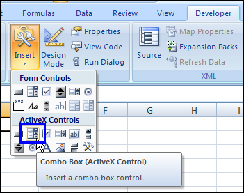
Would you prefer a bigger font size for items in a data validation drop down list?
Could you save typing time, if the words were completed automatically, as you started typing them?