Over at Chandoo’s Excel blog, he’s celebrating VLOOKUP week, with helpful posts like VLOOKUP Formulas Go Wild. Who knew an Excel formula could go wild?
I’ve seen many workbooks where things have run amok, but fortunately, Chandoo’s examples are much better behaved.
Excel VLOOKUP Videos
You don’t need any special equipment or fancy telescopes to do a lookup in Excel — you just need a simple formula.
In my videos below, see how to use the VLOOKUP function, and overcome its few shortcomings with other functions, like INDEX and MATCH.
Watch the VLOOKUP Videos
I’m a big fan of VLOOKUP too, and have made several Excel VLOOKUP videos that show you how to use the function in different scenarios.
Can the sales staff and accounting staff ever work in peace? One group wants to see product descriptions, when entering orders. The other group thinks the descriptions clutter up the worksheet — they just want the product codes.
Try this data validation trick, and you might be nominated for next year’s Nobel Peace Prize. (Results not guaranteed.)
See the workbook details below, and there’s a video with step-by-step instructions at the end of the page.
Create Drop Down Lists
To make it easier for users to enter data in an Excel workbook, you can create drop down lists in the cells, by using Excel data validation.
Excel Drop Down List With Product and Code
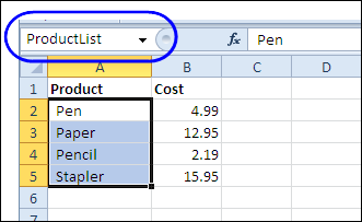
Product Lookup Table
In this example the product list is in an Excel Table, and the ProductShow column is a named range — ProdList.
The ProdList range is used as the source for the drop down lists on the order entry sheet.
Add Excel VBA Magic
After the product is selected from the drop down list, the full description is automatically replaced by the product code. How does it happen?
It’s the magic of Excel VBA — event code that runs when the worksheet is changed.
Drop Down List VBA Code
The Excel VBA code uses the Match worksheet function to find the row number in the lookup list. It replaces the selected product description with the matching Product Code from that row in the lookup list.
Peace at last! Your co-workers will be happy that they don’t have to memorize the product codes, and the accounting department will be grateful that they get the data in the format they need.
Download the Sample File
To see the Excel VBA code that changes the product name to a product code, go to the Contextures website, and download the sample file: DV004: Data Validation Change.
The example used here is the Excel 2007 version, and there is also an Excel 2003 version of the sample file.
Watch the Data Validation Video
You can watch this video to see the steps for creating an Excel Table, naming a column in that table, then using that name when creating the data validation drop down list.
People are lazy! Shocking, I know, but who wants to click twice in Excel, if you can do the same thing by only clicking once?
Click to Sort Column
Peterson, champion of weary Excel users, created this sample Excel VBA sort code, that adds invisible rectangles at the top of each column in a table.
A macro is automatically assigned to each rectangle, and it sorts the table by that column, when you click it.
Benefits of Sort Macros
Here are two benefits of using Dave’s code:
Reduced wear and tear on clicking fingers
Less risk of table scrambling, because it ensures the entire table is selected before sorting
Click Invisible Shapes to Sort Columns
Edit the Setup Macro
There are two macros in Dave’s sample file.
SetupOneTime – run this once, to add the hidden rectangles
SortTable – sorts table by selected column, when heading is clicked
Before you run the SetupOneTime macro, you should edit both macros, to adjust them for your workbook
On the Excel Ribbon, click the Developer tab, then click Macros
Click SetupOneTime, and click Edit
The Setup Macro Code
In the SetupOneTime macro, change the iCol variable to match the number of columns in your table. If your table doesn’t start in cell A1, change that reference.
Edit the SortTable Macro
Next, change the variables in the SortTable macro, to suit your table settings. You can adjust:
TopRow (row where headings are located)
iCol (number of columns in the table)
strCol (column to check for last row)
If you want to see the rectangle outlines, change the Line.Visible setting to True.
Run the SetupOneTime Macro
After you’ve edited the macros, you can run the setup macro:
Select the sheet where your table is located.
On the Excel Ribbon, click the Developer tab, then click Macros
Click SetupOneTime, and click Run
Now, click a heading in the table, to sort by that column.
Excel 2007 Shapes Problem
When I was getting this blog post ready, I discovered that Dave’s original code needed a tweak before it would work correctly in Excel 2007 and Excel 2010.
In the original code, written for Excel 2003, there was one line of code that made the rectangular shape invisible:
.Fill.Visible = False
In the newer versions of Excel, only the borders of the invisible shapes were clickable, so I had to change the code to these two lines:
.Fill.Solid
.Fill.Transparency = 1#
The revised code worked for me in Excel 2003, 2007 and 2010, creating transparent shapes that were clickable.
Download the Sample Workbook
To see the full code for the SetupOneTime and SortTable macros, and download the sample workbook, visit the Sort Data With Excel Macros page on the Contextures website.
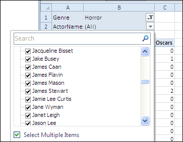
Slasher movies are a scary Halloween tradition, and you can fight back against these horror films, by using Excel Slicers to slash through piles of data.
The Guardian recently posted a list of Greatest Films of All Time. Let’s see how we can use Excel Slicers for Halloween horror films from that list.
To make it easier to people to enter data in your Excel workbook, you can create drop down lists in the cells, by using Excel data validation. These lists will also help prevent invalid entries in your worksheets.
Did you ever get an Excel file from someone else, and try to sort out their Excel VBA code? Or, even worse, open an Excel file that you wrote long ago, and try to remember what all those variables mean?
I spend lots of time staring at Excel code, but apparently I don’t use the right-click menu too often, because I hadn’t noticed a couple of handy commands until recently.
These commands can help you decipher that mysterious code, and unravel the complicated sections.
Excel VBA Quick Info
The first handy command is Quick Info. I have Auto Quick Info turned on in the VBE Editor options, and it helps me remember the syntax as I type the code.
Right-Click for Quick Info
What I didn’t realize was that you can right-click on a variable, function, statement, method, or procedure in the code, and click Quick Info.
Right-Click for Quick Info in Excel Visual Basic Editor
A tooltip appears, with details on the selected item.
Excel VBA Definition
The other right-click command that I finally discovered is the Definition command.
Click the Definition command, and it takes you to the selected variable’s definition.
Finding the definition is easy in most procedures, but in a long procedure, with a long list of variables, the Definition command really makes the job easier.
It’s especially helpful if the variable is defined on a different code module!
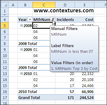
One of the best features of a pivot table is filtering, which allows you to see specific results in your data. See which types of filters are available, and learn how you can apply more than one filter on pivot table field at the same time.
Did you know that you can create waterfalls in Excel — Waterfall Charts? We have a very famous waterfall here in Canada, which you can see in the photo below from our fall vacation, a couple of years ago.
To fill blank cells, or delete rows with blanks cells, you can use Excel’s Go To Special feature.
For example, in the worksheet shown below, you might want to fill in all the blanks in column B, by copying the value from the row above.
There are instructions on the Contextures website to fill blank cells, by using Go To Special to select the blanks.
You can do this manually, and there’s sample code to make the job easier.
Selection Is Too Large Error
This technique works very well, unless you’re trying to fill blank cells in a long list. In that case, you might see the error message, “Selection is too large.”
This happens in Excel 2007, and earlier versions, because there is a limit of 8192 separate areas that the special cells feature can handle. (This problem has been fixed in Excel 2010.)
There are details on Ron de Bruin’s website: SpecialCells Limit Problem.
Work in Smaller Chunks
If you run into this error, you can work with smaller chunks of data instead.
If you’re making the changes manually, select a few thousand rows, instead of the full column.
If you’re using a macro, you can loop through the cells in large chunks, e.g. 8000 rows, instead of trying to change the entire column.
On the Contextures website, Fill Blank Cells Macro – Example 3 checks for the number of areas, using Ron’s sample code, and uses a loop if necessary.
The code is shown below, and it shows a message box if the range is over the special cells limit. You can remove that line — it’s just there for information.
Sub FillColBlanks()
'https://www.contextures.com/xlDataEntry02.html
'by Dave Peterson  2004-01-06
'fill blank cells in column with value above
'2010-10-12 incorporated Ron de Bruin's test for special cells limit
'https://www.rondebruin.nl/specialcells.htm
Dim wks As Worksheet
Dim rng As Range
Dim rng2 As Range
Dim LastRow As Long
Dim col As Long
Dim lRows As Long
Dim lLimit As Long
Dim lCount As Long
On Error Resume Next
lRows = 2 'starting row
lLimit = 8000
Set wks = ActiveSheet
With wks
   col = ActiveCell.Column
     'try to reset the lastcell
   Set rng = .UsedRange
   LastRow = .Cells. _
     SpecialCells(xlCellTypeLastCell).Row
   Set rng = Nothing
    lCount = .Columns(col) _
            .SpecialCells(xlCellTypeBlanks) _
            .Areas(1).Cells.Count
    If lCount = 0 Then
        MsgBox "No blanks found in selected column"
        Exit Sub
    ElseIf lCount = .Columns(col).Cells.Count Then
		   'this line can be deleted
        MsgBox "Over the Special Cells Limit"
        Do While lRows < LastRow
            Set rng = .Range(.Cells(lRows, col),  _
            .Cells(lRows + lLimit, col)) _
             .Cells.SpecialCells(xlCellTypeBlanks)
            rng.FormulaR1C1 = "=R[-1]C"
            lRows = lRows + lLimit
        Loop
    Else
        Set rng = .Range(.Cells(2, col),  _
            .Cells(LastRow, col)) _
            .Cells.SpecialCells(xlCellTypeBlanks)
        rng.FormulaR1C1 = "=R[-1]C"
    End If
   'replace formulas with values
   With .Cells(1, col).EntireColumn
       .Value = .Value
   End With
End With
End Sub

 Over at Chandoo’s Excel blog, he’s celebrating VLOOKUP week, with helpful posts like VLOOKUP Formulas Go Wild. Who knew an Excel formula could go wild?
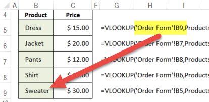
 Can the sales staff and accounting staff ever work in peace? One group wants to see product descriptions, when entering orders. The other group thinks the descriptions clutter up the worksheet — they just want the product codes.