
Remember, Sunday October 17th is Spreadsheet Day, so you’d better start planning your celebrations. You could start the day with a big bowl of Chex cereal — each bite looks like a little spreadsheet. For dessert at the end of the day, have some pie, or bars, while you dream about charts.
Excel VBA – Macro Runs When Worksheet Changed
Are you ready for Spreadsheet Day on October 17th?
Maybe you can add a Spreadsheet Day message to all your workbooks, using the technique described in this blog post.
It’s a macro that runs every time the worksheet changed. I’m sure your co-workers would enjoy that!
Continue reading “Excel VBA – Macro Runs When Worksheet Changed”
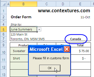
Excel Conditional Data Validation
Happy Canadian Thanksgiving! You probably have your own spreadsheet to organize the meal, but you can download my Excel Holiday Dinner Planner, if you don’t have one of your own.
FLOOR Function – Round Down in Excel
Earlier this week, you read about the Top 100 Canadian Singles, and saw the pivot table that summarized the top songs by decade.
In the comments, Martin mentioned the FLOOR function, that I used to calculate each song’s decade, based on its release year.
File Downloads Fixed
Martin also pointed out that the files weren’t downloading, and I finally managed to fix that — sorry about the inconvenience.
Take my advice, and don’t work on your blog while travelling, if you can avoid it! Things that work perfectly at home, refuse to cooperate when you’re on the road.
FLOOR It
The Excel FLOOR function rounds numbers down, toward zero, based on the multiple of significance that you specify. In the Canadian Music file, the decade is being calculated, so 10 is used as the multiple.
- =FLOOR(A2,10)

In column B, you can see the result of the FLOOR function, rounding down the year for each song, to show the song’s decade.
Trouble on the FLOOR
In the FLOOR function, if the number and multiple have different signs, the result is the #NUM! error. The FLOOR function works well in the music example, because the song’s year is always a positive number.
If you’re working with a list that contains both positive and negative numbers, you could use the SIGN function to calculate the number’s sign, and change the multiple to match it.
=FLOOR(A2,SIGN(A2)*10)

The Excel SIGN function result is 1 for positive number, -1 for negative numbers, and 0 for zero.
Heart of Gold
And finally, for your Friday listening pleasure, here is the second song on the Top 100 Canadian Singles list — Neil Young playing Heart of Gold.
____________
Pivot Table Count Per Decade
 If you’re looking for love, move along — the “Canadian Singles” in the article title refers to hit songs, not eligible bachelors.
Last week, a new book was published with a list of top 100 Canadian singles, based on a poll of music professionals and fans.
In his J-Walk blog, John Walkenbach posted a link to the Canada’s Top 100 Singles list, and there was a lively discussion in the comments section.
Top 100 Canadian Singles List
No discussion is complete without a spreadsheet, so I copied the list into Excel, and cleaned it up.
To make it more interesting, I found the release date for each hit song, and split them into decades, using the Excel FLOOR function.
Make a Pivot Table
From that data, I created a pivot table, showing the count of songs from each decade, listed by rank.
Was most of the best music released in the 1970s, or were most of the voters from that era?

Pivot Table Group Numbers by 10
In column A, the top 100 songs are grouped by 10s, to summarize the data.
For example, row 5 shows the decade counts for the songs ranked from one to ten in the top 100 list.

Highlight with Color Scale
Next, I added conditional formatting to highlight the decades with the largest number of songs.

Repeat Pivot Table Item Labels
A new feature in Excel 2010 pivot tables is the ability to repeat the field item labels.
In another copy of the pivot table, I put the decade in the row label area, and changed the pivot table report layout to Outline Form.

Change Pivot Field Setting
Then, I right-clicked on the Decade field, and clicked Field Settings. On the Layout & Print tab, I added a check mark to Repeat Item Labels, and clicked OK.
After changing that setting, the decade is repeated in each row, instead of showing just once, at the top of the section.

Download the Top 100 Canadian Single File
To see the list, and create your own pivot table, you can download one of my sample files.
- There’s a Top 100 Canadian Singles list in Excel 2007/2010 format
- For earlier versions of Excel, download the Top 100 Canadian Singles list in Excel 2003 format.
_______________
Count Unique Items in Excel Filtered List
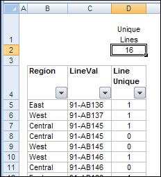
You can use the SUBTOTAL function to count visible items in a filtered list. In today’s example, AlexJ shows how to count the unique visible items in a filtered list. So, if an item appears more than once in the filtered results, it would only be counted once. Thanks, AlexJ!
Continue reading “Count Unique Items in Excel Filtered List”
New Improved Excel Data Entry Form
Many moons ago, Dave Peterson created a sample Excel worksheet data entry form and kindly shared it on the Contextures website.
In Dave’s original form, users could add records on the data entry sheet, and click a button to go to the database sheet, where they could review or edit the order records.
Excel Box Plot Chart-Airport Security Times
 Earlier this month, I had the pleasure of flying out of Chicago’s O’Hare airport. I was checking in at the ungodly hour of 6 AM on a Sunday, and hoped that would be a quiet time at the airport.
Continue reading “Excel Box Plot Chart-Airport Security Times”
Help Improve This Excel Expense Tracker
On the Consumerist website last week, they posted Lauren’s Excel budget template, so I downloaded it, to take a look.
I’d call it an Expense Tracker, rather than a “Budgeter”, because it’s used to record income and expenses. (Do you know the origin of the word “budget”? I had to look it up.)
Expense Tracker Formula
Here’s what it looks like, with part of the formula for the Total cell showing in the formula bar.
The grey fill colour is added with conditional formatting.

Excel Formula for Total
Shown below is the full formula for the Total.
You can see that Lauren has named the date headings (_8_10d) and hidden total row (_8_10) for each month.

So Many Named Ranges
Wow! It makes me tired just looking at that. Lauren created a lot of named ranges, to set up the file, and she’ll need to do more work to add more months.
Because there’s a separate section for each month, her formula needs a SUMIF formula for each range.
She might have to upgrade from Excel 2003, or she’ll pass the character limit for that formula.
Room for Improvement
I don’t know who Lauren is, but she should be commended for setting this up, and keeping track of her income and expenses.
Sure, there are many ways to improve her Budgeter, but it seems to work okay, even if it is a bit convoluted. At least she knows where her money is going!
What Would You Do?
But, there must be better ways to keep track of income and expenses. How would you set up an Excel workbook to do this?
I’d probably create a simple list, with columns for Date, Item, Location, Category and Amount, like the table in the screen shot below.
The last column calculates the year and month, so it’s easy to summarize by month.

Add Drop Down Lists
You could even get fancy, and add data validation to the Category column, with a drop down list of valid categories.
Next, enter all your budget items, then create a pivot table to summarize your spending.

____________
Highlight Winning Lottery Numbers in Excel
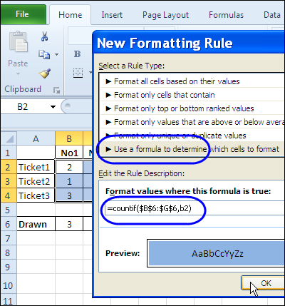
Apparently you have to buy a ticket if you want to win the lottery, so I’m out of luck. However, if you’re in an office lottery pool, or buy your own tickets for the lottery, Excel can let you know if you have a winning ticket.
Continue reading “Highlight Winning Lottery Numbers in Excel”