This week, there were a couple of Excel conditional formatting questions in the blog comments.
- Ron asked about changing the font colour for the highest, second highest and lowest values.
- Guido wants to highlight values that aren’t multiples of another cell’s value.
I’ll answer the questions here, so they’re easier to find. Maybe you’ve encountered similar conditional formatting problems, and this will help.
Change Font Colour for Top 3 Values
The first question is from Ron, who wants to change the font colour, instead of the fill colour:
I am trying conditional format a range of three cells where the FONT of the highest value in the range will be in Red follow by Blue and Green. I know it can be done using cell fill but, with a large spread sheet, it will look like dog’s breakfast. Any help would be appreciated. Also can this be done across worksheets (i.e. three different worksheet in the same file)
Ron didn’t say that the three cells were adjacent, in the same row, but I made that assumption in my example, shown below.

To find the highest, second highest, and lowest values for cells C2:E2 with a worksheet formula, you could do the following:
- To find the highest value, use MAX =MAX($C2:$E2)
- To find the second highest value, use LARGE =LARGE($C2:$E2,2)
- To find the lowest value, use MIN =MIN($C2:$E2)
The column references are absolute, so that all 3 cells in the row will refer to the same range.
You can use the same formulas in conditional formatting, compared to the active cell, and add the font formatting for each formula.
Format the Highest Value
To set up the conditional formatting for the highest value:
- Select cells C2:E6, with C2 as the active cell
- On the Excel Ribbon’s Home tab, click Conditional Formatting, and click New Rule
- In the New Formatting Rule dialog box, under ‘Select a Rule Type’, click ‘Use a formula to determine which cells to format’
- In the formula box, type the MAX formula: =C2 = MAX($C2:$E2) The first reference to C2 is relative, so each cell will check its value compared to the MAX in the $C2:$E2 range.
- Click Format, and on the Font tab, select Red as the font colour, then click OK, twice, to close the dialog boxes.

Now the highest values are highlighted in each row.

Format the Second Highest Value
To set up the conditional formatting for the second highest value:
- Select cells C2:E6, with C2 as the active cell
- On the Excel Ribbon’s Home tab, click Conditional Formatting, and click New Rule
- In the New Formatting Rule dialog box, under ‘Select a Rule Type’, click ‘Use a formula to determine which cells to format’
- In the formula box, type the LARGE formula: =C2 = LARGE($C2:$E2,2)
- Click Format, and on the Font tab, select Blue as the font colour, then click OK, twice, to close the dialog boxes.
Format the Lowest Value
To set up the conditional formatting for the second highest value:
- Select cells C2:E6, with C2 as the active cell
- On the Excel Ribbon’s Home tab, click Conditional Formatting, and click New Rule
- In the New Formatting Rule dialog box, under ‘Select a Rule Type’, click ‘Use a formula to determine which cells to format’
- In the formula box, type the MIN formula: =C2 = MIN($C2:$E2)
- Click Format, and on the Font tab, select Green as the font colour, then click OK, twice, to close the dialog boxes.
Now the highest value in each row is highlighted in red, the second highest is blue, and the lowest is green.

Conditional Formatting From Another Worksheet
To answer the second part of Ron’s question — conditional formatting won’t let you refer to cells on a different worksheet, or in a different workbook.
However, you can refer to a workbook level named range that’s on a different worksheet, but that wouldn’t help in the example shown above.
For example, you could highlight all the cells on Sheet1 that are higher than the maximum allowed, if the maximum is on Sheet2, in a range named MaxAmt.
=C2>MaxAmt
And here’s another example of referring to a named range in conditional formatting.
Highlight Cells That Are Not a Multiple of Another Cell
The next conditional formatting question came from Guido:
need conditional formatting based on the multiple of the number oin another cell. How to do that?
For ex: in the formatted cell can only be the multiple of the number in the other cell, otherwise it colours for ex red
To check this on the worksheet, you could use the MOD function:
=MOD(D2,C2)
The MOD function returns the remainder after a number is divided by divisor. If the result is zero, then D2 is a multiple of C2.
Highlight the Non-Multiples
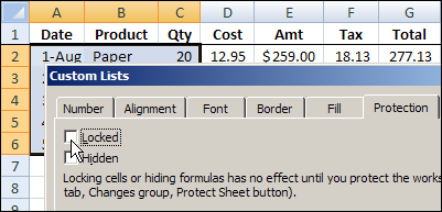
Shown below is the sample data for this conditional formatting example.

To add the conditional formatting, and highlight the non-multiples in column D:
- Select cells D2:D6, with D2 as the active cell
- On the Excel Ribbon’s Home tab, click Conditional Formatting, and click New Rule
- In the New Formatting Rule dialog box, under ‘Select a Rule Type’, click ‘Use a formula to determine which cells to format’
- In the formula box, type the MOD formula: =MOD(D2,C2) <> 0
- Click Format, and on the Fill tab, select Red, then click OK, twice, to close the dialog boxes.
Now the non-multiples in column D highlighted in red.

More Excel Conditional Formatting Examples
There are more Excel conditional formatting examples on the Contextures website.
______________


 Last week, I posted Bob Ryan’s Excel macro for
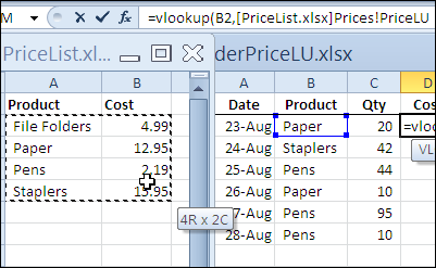
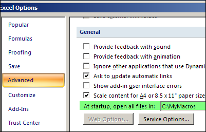
 Do unwanted files open automatically when Excel starts? Perhaps something changed in your computer, and Excel files are opening automatically, and you want to get rid of them. Keep reading, to see where those files might be located, and how to stop them from opening.