
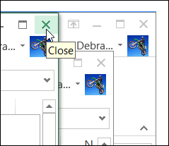
One of the new features in Excel 2013 is that each file opens in a separate window. Having each file in its own window makes it easier to compare files side-by-side, and most of the time I like the separate windows.
Category: Excel tips
Show RSS Feeds on Excel Worksheet
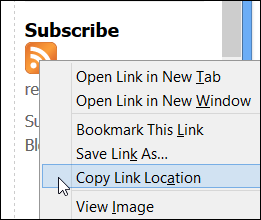
As you’ve heard, Google Reader will be disappearing in a few months <sigh>, and we’ll have to find other ways to follow our favourite blogs. I’m looking for a replacement, but haven’t found anything perfect yet. How about you?
Go Back to Previous Locations in Excel
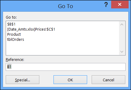
In Excel, you can create named ranges, and go to those ranges by selecting a name from the Name Box.
Excel Date Picker Tool
If you’d like a quick and easy way to add dates in a worksheet, you can use this handy date picker tool, from Jim Cone.
The Date Picker opens to the current date, and you can scroll through months and years, by using the scrollbars at the top of the date picker form.

Just select a cell, and click the insert button, to add the date. If you hold the Shift key, and click the Insert button, it will append the date to the cell’s contents.

Create Calendars on a Worksheet
In addition to inserting the date, Jim’s date picker will also add a calendar to the worksheet – either a single month, or a full year.

Download the Date Picker File
To see all the details, and to download the date picker file, please visit my Contextures website: Excel Date Picker
The file is in Excel 2003 format, and contains macros, so enable macros if you want to test the file. The VBA code is unlocked, so you’ll be able to poke around in the code, and see how it works.
Jim hasn’t tested the file in Excel 2013, but a quick test in that version worked fine for me.
__________________
Show File Open Window in Excel 2013
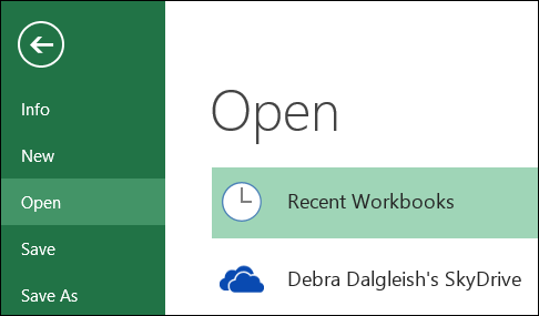
In Excel 2013, if you click the File tab, you go to the Backstage view. The Open command is selected, and you can select a file and open it.
Add Custom Ribbon Tab For Workbook
Last week, you saw how to open and edit the Ribbon code in an Excel file that has a custom tab. This week, you can see how to create a custom tab in an Excel workbook, and add buttons to run your macros.
This example is based on an Order Form workbook, and the buttons run macros to clear the data entry cells, and to view the file before printing.

You’ll see how to set the custom tab labels and icons, and change your macros so they run from a click on the Ribbon. Exciting, right?
Watch the Video
To see the steps, please watch this video. It’s a bit longer than the videos that I usually make, but the steps are quite easy, so give it a try!
Download the Sample File
To see the written instructions, and to download the sample file, please visit my Contextures website: Add Custom Ribbon Tab to Workbook
Excel Dashboard Course Re-opens
Custom ribbon tabs can make your workbooks easier to use, and they add a professional touch. If your goal is to build a dashboard, Mynda Treacy from My Online training Hub is opening her Excel Dashboard Course, and if you sign up by January 30th, you can get it for 20% off.
The course is video based, delivered online and is available 24/7. You also receive comprehensive workbooks and sample dashboards to keep. There’s even an option to download the videos.
The previous classes were very successful, and you can read the glowing reviews from the students, who loved all the techniques that they learned in the course, and are using them to impress their colleagues.
Click here to find out details of the course, read the student comments, and watch the ‘behind the scenes’ video that shows you what you’ll receive as a member.

________________
Open Excel 2013 With Blank Template
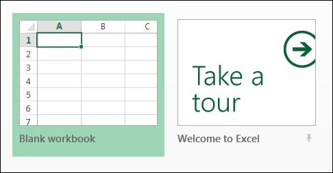
If you’ve been using Excel 2013, you might enjoy seeing the collection of templates when you open Excel. There is a blank template at the top left, and you can even take a tour of Excel.
Keep Numbers Aligned When Zooming
Who knew that this would still be a problem in Excel 2013? Almost 4 years ago, I posted about numbers not lining up, when Excel was zoomed to less than 80%
Now I’m working on a new laptop, and realized that the problem is back. In Excel 2013, I’m using the default font – Calibri 11. Here’s a list of numbers, at 80% zoom.

And here is the same list at 72% zoom – the numbers have changed to a proportional font, and the 1111111s are much narrower than the 8888888s.

Change the Registry
To fix the problem, I followed the instructions that I posted in April 2009, when I was setting up my previous laptop. Here they are again, with adjustments for Windows 8 and Office 2013. The original instructions came from this MSKB article:
Euro Currency Character Is Not Displayed Correctly in Excel 2003
This is really a fix for a Euro symbol display problem, but it also fixes the proportional font display.
Steps to Fix Problem
Here’s what I did for Win8 and Excel 15:
- Make a backup copy of the registry before you tweak any settings
- Quit any programs that are running.
- Press the Window key and R, to open the Run window.
- In the Open box, type regedit, and then click OK.

- Locate, and then click to select the following registry key:
HKEY_CURRENT_USER/Software/Microsoft/Office/15.0/Excel/Options - With the Options key selected, point to New on the Edit menu, and then click DWORD (32-bit) Value.

- Type FontSub, and then press ENTER.
- Right-click FontSub, and then click Modify.

- In the Value data box, type 0. Since the value is zero, it doesn’t matter which Base you select – I left it on Hexadecimal.

- Click OK to close the Edit DWORD window
- On the File menu, click Exit to quit Registry Editor.
- Start Excel, and the numbers should line up correctly, eve when zoomed.

___________________
Add Picture to Excel Comment
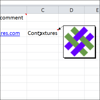
Things have been hectic this week. I got a new laptop, with Window 8, and have spent hours installing software, and getting all my settings the way I like them.
I’ve also installed the latest version of Excel 2013, and am using it for my daily work, so there’s lots of new stuff to play with and learn.
Continue reading “Add Picture to Excel Comment”
Spreadsheet Day 2012
Do you have your party plans finalized? Remember, tomorrow, October 17th, is Spreadsheet Day, in honour of the date that VisiCalc was first shipped.
Last year, the theme was spreadsheets for students, and I posted a student time tracker in which you can plan your projects and track your class and lab hours.
![]()
In 2010, I posted my top 5 Excel tips, that I had seen posted on Excel blogs over the previous year. One of those tips was Jon Peltier’s tutorial on making vertical bullet graphs.

Top 5 Excel Tips for 2012
This year, I’m going back to the top 5 theme. Every week, in my Excel News email, I link to interesting articles that I’ve found on other blogs. Some are simple tips, others are more complicated, and some are food for thought.
Below, in no particular order, are my favourites from those articles. And if you’re not on my Excel News mailing list, please add your name, by using the form at the top right.
VBA Conditional Formatting of Charts by Value and Label
Jon Peltier, who creates time-saving Excel chart utilities, shared his technique for building charts with conditional formatting that is based on the values and labels.
In the screen shot below, the Beta bar is dark red, because its value is high, and the Alpha bar is very light blue, because its value is low.

Force Clients to Enable Macros
If you’re creating automated workbooks for other people to use, you might run into problems if those people don’t click the button to enable the macros. That macro warning can be easy to overlook, or it might not even appear, if security level is set to High.
[Bacon Bits blog is no longer online]
Mike Alexander, in his Bacon Bits blog, explains how he solves the problem, by Forcing Your Clients to Enable Macros. Users can’t miss the giant message in his workbooks, and they can’t do any work until they enable macros.

Who Says the Ribbon Is Hard?
Bob Phillips convinces us that it’s easy to make dynamic changes to the Excel Ribbon. In his article, Bob explains how to use Excel VBA to change the Ribbon commands.
He shares his sample code, and you can click the link to download his sample workbook. The link opens as an Excel Web App, so click the File tab, then click Download a Copy, to save a copy on your computer.
Create an Interactive Sales Chart
Chandoo posts hundreds of great Excel tips on his blog, so it was hard to pick just one for this list of favourites. However, I finally selected this interactive sales chart example, because it incorporates several useful techniques.

You can use Chandoo’s example to build your own dashboard with a dazzling interactive chart. Download the sample file, and poke around in the code, to see how it works.
Microsoft Excel Check List Template
On his Clearly and Simply blog, Robert Mundigl has created an Excel template for a structured Checklist. It gives you the option to check and uncheck by double clicking.
That’s a feature that many people like, so you can use download the Microsoft Excel Check List Template and use the same technique in your workbooks.

What Are Your Favourite Excel Tips?
It was tough to pick a top 5 Excel tips, and I’m sure there are many other tips that you found. If you have favourite articles from the past year, please share a link in the comments below.
____________