
 If you have the day off, you can spend some time playing this Excel Treasure Hunt game. Or, if you celebrate Easter, give this to your kids — it’s cheaper and easier than hiding chocolate eggs!
Author: Debra Dalgleish
Dependent Data Validation From Pivot Tables
 Cascading lists and kangaroos? Today, Ed Ferrero shares his technique for creating dependent data validation from pivot tables. Ed’s from Australia, and it looks like we’ll learn a bit about his country too, as we go through his sample file.

Dependent Data Validation
We’ve created dependent data validation drop downs before, based on named ranges, or sorted lists. Ed’s technique is perfect if you have a large data source, and it isn’t sorted in the order that you need.
In this example, there’s a list of States and Cities, with the cities in alphabetical order.

Create the Pivot Tables
Ed created two pivot tables, one with State in the row area, and one with State and City in the row area.

The State labels don’t repeat in the pivot table, so you can’t use the sorted table dependent data validation technique.
Create the Named Ranges
Instead, Ed created a couple of named ranges, and some dynamic ranges.
- The first range is State, which is the list of state names and Grand Total in the first pivot table.
- The second range is StateCity, which is the list of state names and Grand Total in the second pivot table.
Tip: If you reduce the worksheet zoom to 39%, you can see the range names.

Create the Dynamic Ranges
The first dynamic range is for the City heading in the second pivot table.
- CityHeader: =OFFSET(StateCity,-1,1,1,1)
The next two dynamic ranges, StateNo and StateCityNo, use relative references to read the value of the state from the cell to the left of the active cell. For example, if the selected State is in cell A3 on Sheet1, these formulas are used:
- StateNo: =MATCH(Sheet1!A3,State,0)
- StateCityNo: =MATCH(Sheet1!A3,StateCity,0)
Queensland is the selected State, so StateNo =3 and StateCityNo =5.
Then, the next State is found in the StateCity range.
- StateCityNext: =MATCH(INDEX(State,StateNo+1),StateCity,0)
The next State is South Australia, and it’s in row 9, so StateCityNext =9.

Create the Dependent List of Cities
Finally, the dynamic range for the list of cities is created.
- City: =OFFSET(CityHeader,StateCityNo,0,StateCityNext-StateCityNo,1)
The City range is offset from the CityHeader cell, 5 rows down, 0 columns right, 4 rows high (9-5), and 1 column wide.

Create the Drop Down List
The final step is to create the data validation drop down lists. In cell A3, a State drop down list is created, based on the State range.

In cell B3, a dependent City drop down list is created, based on the City range.

Download the Sample File
You can download Ed’s sample file to see how it works: Dependent Data Validation From Pivot Tables. It’s a zipped file, in Excel 2003 format.
About Ed Ferrero
Ed maintains an Excel techniques web site at www.edferrero.com. He is based in Australia, and has been a Microsoft Excel MVP since 2006.
____________
Track Your Treatments in Excel
 Don’t get too close to this blog today – I’ve got a miserable cold, and wouldn’t want you to catch it!
Roger Govier has created an Excel file to track your medical treatments, for people who have varying dosages or injection sites. It won’t help me feel better, but it might help you, or someone you know.
Enter the Treatment Sequence
Roger’s workbook has two worksheets – Calendar and Setup. Start on the Setup sheet, where you’ll enter the medication sequence.
First, enter your daily dosages in the Treatment List column.
- For example, someone who’s taking a medication might be prescribed to take daily doses of 2 mg, 2mg, 3mg, 2mg, 5mg and then back to the start of the sequence.
- They would fill in 5 cells in the Treatment List, shown in section 1 in the screenshot below.

Next, after you’ve entered the daily dosage sequence in the Treatment List, click the Fill Treatment Column button (number 2 in the screenshot above).
A macro runs, which clears the Treatments column (number 3 in the screenshot) and then fills it again, based on the treatment sequence that you entered.
View the Treatment Calendar
After setting up the Treatment Sequence, go to the Calendar sheet, which shows a monthly calendar.
At the top of the worksheet, select a year and month from the drop down lists.

Then, from the Start Treatment drop down, select the starting treatment for the selected month. In this example, the previous month ended with a 3mg dosage, so the fourth dosage, 2mg, is selected.

The calendar automatically adjusts to show the new treatment schedule.
Download the Sample Treatment Workbook
Click here to download Roger’s Sample Excel Treatment Workbook. It’s a zipped file in Excel 2003 format, and contains a macro.
You’ll have to enable macros to run the FillColumn macro on the Setup sheet.
Healing Music
If you’re sick too, this video, with the soothing sounds of Peggy Lee, might help you feel better, and get rid of your fever.
______
Old Excel Dogs Learn New Tricks
 Yes, if your last name is Dalgleish, some people think it sounds like “Dog Leash”, and hilarity ensues. And no, I never get tired of that joke, thanks for asking. 😉
Anyway, unlike the proverbial old dog, those of us who have been using Excel for a long can CAN learn new tricks. Keep reading to discover which new Excel feature I recently discovered.
Long Time Excel Users
Maybe you’re a long time Excel user too. Last month I polled readers on my Debra D’s Blog, and asked How Long Have You Been Using Excel?
Almost half of the 80 respondents have used Excel for 16 years or more, and they shared some interesting stories in the comments.

Old Excel Habits
You learn a lot about Excel over the years, and appreciate both its strengths and limitations. You find workarounds for some of the features that don’t work the way you’d like, and accept that some things can’t be done in Excel.
Maybe you’ve even learned to love (tolerate?) the Excel Ribbon, despite all the years that you spent learning where the Menu commands were.
But occasionally, new features are added, without much hoopla, and you don’t even notice them. At least, that’s what happened to me!
Old Excel Header Tricks
Excel has customizable headers and footers, where you can place items like the date, or file name, in one of three sections — left, centre or right.
On the Excel Ribbon, click the Insert tab, and click the Header & Footer command, to change to Page Layout view, with the Header activated.

See Header and Footer Tools
While the Header or Footer are activated, there’s a Design tab on the Ribbon, with Header and Footer tools.
You can click on an Element, like Page Number, to add it to a section in the Header or footer.

Or, select one of the default options from the Header or Footer drop down lists.

The Page Layout wasn’t available in previous versions of Excel, but the Header and Footer Elements are pretty much the same as they’ve always been.
New Excel Header Tricks
After working with Excel 2007 for almost three years, I finally noticed that the Excel Header and Footer have some fancy new Options. (How embarrassing!)
Now you can have a different header/footer on the first printed page, and different header/footer on the odd and even printed pages.

So, you could show a title on the first page only, then have page numbers at the left on even pages, and on the right on odd pages.

Microsoft Word has always had these options, but Excel didn’t. We just accepted that “Excel isn’t a word processing program” and did without the header options.
Align Header and Footer
You can also align the Excel Header and Footer with the page margins, which is another nice feature. In the old days, the Header and Footer margins couldn’t be changed, so they sometimes looked a bit out of line with the rest of the printed page.
Here’s the Page Layout view, with the Align With Page Margins feature turned on.

I hope you found these new Excel Header and Footer options long before I did, and remember to use them in your printed worksheets.
__________
Select Answers With Excel Option Buttons
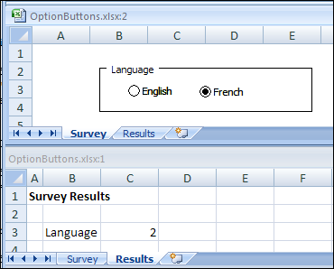
 Male or female? English or French? Yes, No or Maybe? Those are just a few of the choices that you can make with Option Buttons in Excel. When people select answers with Excel Option Buttons, you can provide a list of possible answers to a questions, and users can only select one answer from the list.
Calculating Rank in Excel
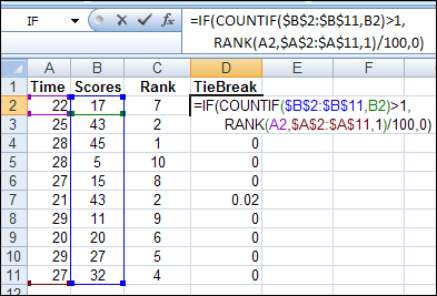
To do some research on sorting, I hauled one of the big, dusty Excel books off my shelf, to see if there were any scintillating sorting secrets to uncover. Under Sorting, I saw “rank calculations” so I turned to that page, to see what it said about calculating rank in Excel.
Number Visible Rows in Excel AutoFilter
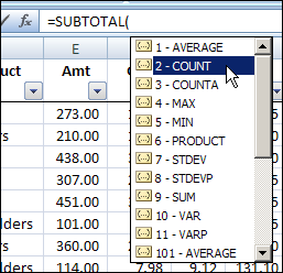
When you create a list in Excel, do you start with a column that numbers the rows? I usually create an ID column and type the number, or use a formula to automatically number them.

In the steps below, I’ll show you the simple numbering system. There’s a fancier formula too, if you’d like to see consecutive numbers when the list is filtered.

Excel Irish Flag St Patrick’s Day Excelebration
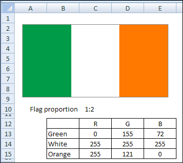
Sometime in the 1840s, probably because of the famine, my dad’s ancestors left Ireland, and boarded a ship to Canada.
The details are sketchy, but I’m sure they had first class accommodations, and sat at the Captain’s table every night.
Continue reading “Excel Irish Flag St Patrick’s Day Excelebration”
Edit Records in Excel Worksheet Data Entry Form
How can you make it easy for people to enter and edit data in Excel, but keep them away from the data storage worksheet?
Last year, I posted a Worksheet Data Entry Form in Excel, where users could enter and view Excel data. It was based on a worksheet data entry form that Dave Peterson created.
I’ve created a new version, where users can enter, view and edit the Excel data.
Version 1: Add New Records
In Dave’s original worksheet data entry form, users could add records on the data entry worksheet, and click a button to go to the database sheet, and review or edit the order records.

Version 2: View Existing Records
In version 2, I added a few buttons to Dave’s workbook, to allow users to scroll through the existing records.
With the navigation buttons, you could go to the first, previous, next or last record, or type a record number, to go to a specific record.

Version 3: Update Existing Records
In the latest version of the Excel Worksheet Data Entry form, I’ve added an update feature.
As in the previous version, there are data validation drop down lists, to select Item and Location.
The Price calculation is based on a VLOOKUP formula, and the Total formula multiplies the quantity by the price.
After you select a record, you can change its data, then click the Update button to copy those changes to the database.

For example, in the record shown above, if you discovered that there was an error, you could change the quantity from 500 to 200. The Total formula would automatically recalculate, to show the new total of $200.00.
Then, click the Update button, and the revised quantity and total would appear in that record on the database sheet.
The Update Code
Before updating the database record, the Update code checks to see of all the data entry cells are filled in. If they aren’t, a warning message appears, and the macro stops running. This prevents you from accidentally overwriting an existing record with blank cells.

If all the data entry cells are filled in, the code:
- writes the current date and time in the applicable row of the database
- adds the User Name from the Excel application
- copies the data to the database
- clears the data entry cells
Then, with a cleared data entry sheet, you can go on to add, view and edit other records, or save and close the workbook.
Download the Sample File
The zipped sample workbook, in Excel 2003 format, can be downloaded from the Contextures website: Worksheet Data Entry Form
___________
Go Undercover With Hidden Excel Worksheets
 An Excel workbook certainly isn’t Fort Knox, and the information you store there isn’t too secure. If someone opens your Excel workbook, and is determined to see everything in there, they’ll probably be able to.
However, if your goal is simply to make a workbook easier for people to use, you can hide some of the worksheets, so users don’t accidentally change their contents.
For example, if your data entry worksheet has data validation drop downs, you can store the lists on a different sheet, and hide that sheet.
Hide an Excel Worksheet
To quickly hide a worksheet in Excel 2007, right-click on the sheet tab, and click Hide.

If you’re using an earlier version of Excel, activate the sheet that you want to hide. Then, click the Format menu, then click Sheet, and click Hide.

Show an Excel Worksheet
To show the hidden sheet again, right-click any sheet tab, then click Unhide. (In earlier versions of Excel, click the Format menu, then click Sheet, and click Unhide.)

In the Unhide dialog box, click on a sheet name, and click OK.

Really, Really Hide an Excel Worksheet
If you want to hide a worksheet a little better, you can use a special technique that keeps it from appearing in the Unhide list.
- First, to open the Visual Basic Editor (VBE), press the Alt + F11 keys.
- In the Project Explorer, at the left of the VBE window, locate your workbook.
- In the Microsoft Excel Objects folder for your workbook, click on the sheet that you want to hide
- If the Properties window is not showing, press the F4 key to open it
- At the bottom of the Properties window, in the Visible property, change the setting to -2 – xlSheetVeryHidden
- Close the VBE and return to Excel

The sheet is now hidden, and its name won’t appear on the Unhide list.
Watch the Excel Hidden Sheets Video
To see the steps for hiding Excel worksheets, you can watch this short Excel video tutorial.
______________