Lots of people visit my Contextures website looking for information on the Excel Count functions.
Counting seems like an easy thing to do in Excel, if you’ve been using the program for a while. But, if you’re just starting out, it might not be so obvious.
Count Quirks
Even if you’re an experienced Excel user, there are a few quirks with the Count functions, that you might not have noticed yet.
For example, different count functions treat “empty” cells differently, as you can see in the screenshot below.
In Row 5, the blue cells contain a formula that creates an empty string.
The COUNTA function counts that cell, even though it looks empty.
The COUNTBLANK function counts the cell too, even though it contains a formula.
There are many more tips, examples and videos on the Excel Count functions page on my Contextures site.
Video: 7 Ways to Count in Excel
To see a quick overview of 7 ways to get a total count of cells in Excel, watch this 77-second video. There are written steps for each count function on the Excel Count functions page.
When you summarize data in a pivot table, it usually shows a sum of the values. (If there are blanks or text values in the field, usually the pivot table shows a count instead.)
In this pivot table, you can see the total labour cost for each Service Type.
If there are two or more fields in the Row or Column area, subtotals are automatically created for all the fields except the last one.
In the screenshot below, the District field was added below the Service Type field. Subtotals were automatically added to Service Type.
Change the Summary Function
Instead of seeing the Sum of the data, you can change the summary function, and show the Average, or any of the other options. You could even put the same field in the Values area of a pivot table multiple times, and use different summary functions in each column.
In this example, the sum of the labour cost is shown in column C, and the Max function is used in column D.
Subtotals for Sum and Max
Change the Subtotal Summary Function
If your pivot table already has lots of columns, you might not want to make it wider, by adding another copy of one of the Value fields.
Instead, you can change the summary function for the Subtotal, so it uses a different function than the Value fields.
Now the Value fields show the sum of labour costs, and the subtotal for each service type shows the highest labour cost that was charged for that service.
You can see the maximums, without adding extra columns to the pivot table.
More Info on Pivot Table Subtotals
You can read more about pivot table subtotals, and the steps for changing them, on the Contextures website: Excel Pivot Table Subtotals.
Watch the Pivot Table Subtotals Video
To see the steps for changing the pivot table subtotals, and creating multiple subtotals, you can watch this short video.
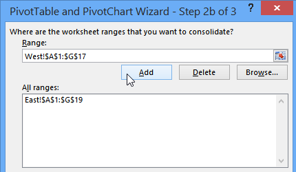
If Excel data is on different sheets, you can create a pivot table from multiple sheets, by using multiple consolidation ranges. My video, further down this page, shows you the steps.
Of course, it’s better if the data is all on one sheet. But, if you don’t have that option, the multiple consolidation ranges will pull all the data into one pivot table.
There’s a sample Excel workbook on my Contextures website that uses a bit of Excel VBA to automatically add new items to an Excel data validation drop down list.
Add New Item to List
For example, if the drop down list shows Apple, Banana and Peach, you can type Lemon in the data validation cell.
Then, as soon as you press the Enter key, Lemon is added to the named range that the data validation list is based on.
The source list is sorted too, so that Lemon appears between Banana and Peach.
New item added to data validation drop down list
Read the Instructions
Someone emailed me last week, and asked if I would explain how the Excel VBA code works.
It rained (and even snowed a little) on Friday, so it was a good day to stay in, and work on a new page for the website.
When printing Excel comments as displayed, you can either show all the comments, or just show one or more comments that you want to print.
To show all the comments, on the Ribbon’s Review tab, click Show All Comments.
Show All Comments
Show Specific Comment
To show a specific comment, select a cell that contains a comment. Then, on the Ribbon’s Review tab, click Show/Hide Comment.
Arrange Comments for Printing
If necessary, rearrange the comments, so they don’t overlap, or cover the data.
Arrange Comments for Printing
Page Setup Dialog Box
Then, on the Ribbon’s Page Layout tab, click the More button for Sheet Options
In the Page Setup dialog box, on the Sheet tab, select As Displayed on Sheet from the Comments drop down.
Page Setup Dialog Box
Quick Check With Print Preview
If you want to see how the comments will look when printed, click Print Preview
Click OK to close the Page Setup dialog box.
Print Comments at the End
Instead of printing the Excel comments as displayed, you can print them at the end of the worksheet.
On the Ribbon’s Page Layout tab, click the More button for Sheet Options
In the Page Setup dialog box, on the Sheet tab, select As Displayed on Sheet from the Comments drop down.
If you want to see how the comments will look when printed, click Print Preview. The comments and their addresses will appear on a separate sheet, at the end of the worksheet’s data.
Click OK to close the Page Setup dialog box.
Watch the Video
This Excel Quick Tips video shows how to display all the worksheet comments, and then print the worksheet with the comments displayed.
“In the back of my mind, I always knew that charts would help me,” says the market researcher in this promotional video from 1982. Wow, did you really have to wait weeks for your data processing department to make your charts, back in the old days?
It’s easy to hide rows and columns in an Excel worksheet, and you or your boss or co-worker might do that when setting up an Excel file.
Occasionally though, you might have trouble unhiding Excel row and columns. There are written steps and a video below, that show how to fix the problem