Dynamic Excel Named List Grows Automatically

Dynamic Excel Named List

You can quickly create a named range in Excel, but it doesn’t automatically expand to include new items that are added at the end of the list.

However, a dynamic Excel named list grows automatically, so here’s how to create that type of list.
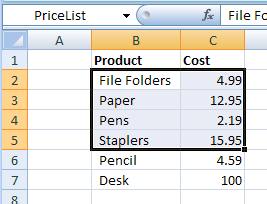
static list doesn't automatically expand to include new items
static list doesn’t automatically expand to include new items

Create a Dynamic Named Range

If you plan to add new items to a list, create a dynamic named range, by using an OFFSET formula.

Here are the steps:

  • On the Ribbon, click the Formulas tab
  • Click Define Name
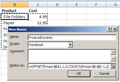
  • Type a one-word name for the range, e.g. PriceListDynamic
  • Leave the Scope set to Workbook.

Add the Formula

Next, in the Refers To box, enter an Offset formula that defines the range size, based on the number of product names in column B

In this example, the following OFFSET formula is entered in the Refers to box:

=OFFSET(Prices!$B$1,1,0,COUNTA(Prices!$B:$B)-1,2)

How It Works

Here’s how the OFFSET formula works:

  • Using cell B1 as the reference cell, the list will start 1 row down, and 0 columns to the right.
  • It counts all the items entered in column B, and subtracts 1, because the list won’t include the heading in B1.
  • The list will be 2 columns wide.

namedynamic02

Then, as new items are added to the list, the dynamic named range will automatically expand to include them.

Video: Dynamic Excel Named List

To see the steps for creating a quick named range and a dynamic named ranged, you can watch this video tutorial.

_______________

41 thoughts on “Dynamic Excel Named List Grows Automatically”

  1. Hi Debra:
    I like the idea of using a Dynamic Named Range, however, for the workbook that I am using now, this range is in the middle of the sheet, with data above it.
    Is there a way to handle a situation like this.
    Thanks – I appreciate your insights into Excel, I use your tips all of the time.

  2. Hi Stan, if you know which row the range starts in, you could subtract everything above that. For example, if the range starts in B31, and that position won’t change:

    =OFFSET(Prices!$B$1,30,0,COUNTA(Prices!$B:$B)- COUNTA(Prices!$B1:$B30),2)

    Or, name the start cell for the range, and use that to find and count the cells above it:

    =OFFSET(Prices!$B$1,ROW(StartCell)-1,0,COUNTA(Prices!$B:$B) – COUNTA(OFFSET(Prices!B1,0,0,ROW(StartCell)-1,1)),2)

      1. Following on from this, when I use a dynamic range to pick information from the middle of a table of data I get no column headers when I reference the named range in a Pivot Table – I’ve tried selecting the first row and the named range as a source for the Pivot and even using both the first row and the dynamic formula as a named range but neither work.
        I’ve been searching for days and can’t find any information on how to do this.
        Please help! 🙂

      2. @Dan, you won’t be able to create a pivot table from data in the middle of a range. Perhaps you could use an Advanced Filter to extract the data to a different worksheet, and base the pivot table on the extracted data.

  3. I love these and use them a lot, but recently I have been rethinking how much I use them. Typically I use these together with a list via data validation so that the drop-down list updates appropriately. But then I found out that using a dynamic range doesn’t restrict user entry in the cell. If you have a hard coded range, then you can set up data validation to only accept items in that list. If you try to type anything else, it will throw an error and tell you to fix it. With dynamic ranges, you can type whatever you want in the data validation cell, even if it doesn’t match the list, and you will get no error.

    Annoying.

  4. Jayson, the data validation lists based on a dynamic range should block any invalid entries, unless there’s a blank cell in the dynamic range. Check your formula to make sure you aren’t including an extra row.

  5. Debra- That was my thought at first. Would you care to try and let me know what you find? I’ve just tried again tonight. I don’t see a blank row (no blanks in the data validation drop-down).

  6. Debra,
    I totally agree with your post. Since I first know of this thanks to Chandoo’s post, I have never stopped using it.

    Stan, maybe you’d like to consider split the contents of your sheet in 2 different ones: one with the data and one with the summary or the remaining contents. It helped me on structuring both macros and formulas, and it’s easier to understand and maintain by someone else if the chance arises, proving your professionalism.

    Rgds,

    Martin.

  7. Martin, you’re right, separate sheets certainly make things easier to maintain.

    Doug, thanks for the link! That’s a nice solution to the problem of deleted heading rows.

  8. One problem I have with dynamic name lst is when I create a pivot table using query (to combine various sheets), these names does not seem to be recognised by MS Query.

  9. HI Debra, I need to do the same thing but instead of adding rows to columns, I need to dynamically add columns to a single row. For example, column A starting in cell 1 has 25 rows of time intervals. Each day I need to add the previous days numbers to the next empty column. I have that figured out, but I would like to use a named range for each of the 25 rows and have them dynamically expand as I would like to use the named ranges in reports I have created based on this data. So each row must have it’s own unique named range that expands across columns. Can you use a variation of the code above to accomplish this? if not, can you shed some light on how it might be done. Love your site, thanks

  10. @Boon, you might have to use a non-dynamic named range, and use a macro to redefine the range after you’ve added or deleted data.

    @wayne, you can use a COUNTA function to calculate the number of columns too. For example, count the cells with data in row 1:

    =OFFSET(Prices!$B$1,1,0,COUNTA(Prices!$B:$B)-1,COUNTA(Prices!$1:$1))

  11. Does anybody use Data>Lists (or Tables in 2007) for dynamic data validation lists? I’m just fooling around with it. After creating the List, I created a named range, using only the column of the list that I want in the data validation, and excluding the header.

    This seems to work well, with the following benefits:
    – Can have more than one list on a Validation Lists worksheet (each one having its header in Row A) and am only allowed to insert/delete rows from one List at a time. (With more than one dynamic range on a sheet it’s easy to accidentally delete a whole row spanning multiple ranges.)
    – Am prevented from deleting a list’s header row.
    – The named range expands and contracts with the list as I add or delete rows, just like a dynamic range.
    – The data validation range isn’t affected if you add other items below the List in the same column.
    – Deleting all the items in the list results in a blank as the only data validation choice – the named range adjusts to include the “*” row of the List. However, when I add items back in the List, the “*” row is no longer included, and the blank Data Validation choice goes away.
    – the named range is visible in the Name box

    I’d be interested to know if people use this method. I don’t recall seeing it mentioned.

  12. Doug, the List and Table features certainly have many benefits, as you mentioned. However, many of my clients still have some people using Excel 2002 or earlier, so I can’t risk using those features, since they aren’t supported.

  13. Thanks Debra. After I posted my comment I realized that I’m only working with 2003 or later right now, but that the issue is exactly what you said for earlier versions. Other than that, Lists/Tables seem to work very well in place of dynamic ranges for DV. I’ve written some VBA code to convert a range to a List and then add a named range to the first column for this purpose.

  14. Hey Debra

    Great post, I have a question though and at the risk of being asking one too complicated for a comment…..

    What I would like to do is have primary and dependent lists that update automatically. The primary list is a list of phases, the dependent list is a list of sub phases. The user chooses a phase in column A, which then dictates which list they will choose from in column B. I want users to be able to add/edit/delete both phases and sub phases as they see fit since this is a living document. They way I am doing it now is through a recorded macro that uses insert>name>create, but it adds all the empty cells to the list.

    Thanks for any help
    Johannes

  15. Dear Debra,
    My name is joju andi am working in a construction company i would like to learn step by step for applying dinamic name range i have some datas of employees like

    Code no Name Designation
    2343 Mr.A Construction Manager
    2345 Mr. B Project Engineer

    Like this the data base will be added with new code no and employees in thease cases how can i use dinamic name range

  16. Hello, we use excel to record employee time worked. When a employee works over 40 hours in a given week, we require a formula that will distinguish when the total hours total over 40 and place that (additional over 40) value into a different cell which will then calculate time and a half of pay for each hour of over time.

  17. Dear Debra—
    First of all, I love dynamic ranges, and have used them in the past, but this time is different, and I have no clue how to approach this “challenge”. I am pulling data from Cognos and linking it within Excel to perform various calculations. Now the report I have has a total of 105 rows of data and 19 columns. These 105 rows of data include “header” rows to seperate the data by location and then by person. I need to be able to link data based on both the location and then the person. A dynamic range does not appear to be something that would work because the way my data is. The number of rows would vary earch time the report is run, but the number of columns will remain consistant. Any ideas Since there is no “dead space” between each location’s data?
    I can probably recreat my Cognos report to list each location on a seperate page (which would be a seperate tab within Excel), but would I need to set up a range for each column (remember there are 19) within each location (there are about 12)? Any assistance you can offer would be greatly appreciated!

    1. Sherry,
      You may still be able to use dynamic ranges. First, create a dynamic range for the whole column with Location names so you can search for Locations in that range. Assuming you have a fixed set of Location names, you could use the MATCH function to find the starting row for each Location to determine the row offset, then you could use MATCH to find the top row again and subtract it from the start row of the next Location (using MATCH for the 3rd time) to get the height of the range. Depending on how you define the start row you’ll probably need to subtract 1 more from the range height. You’ll also need to add a dummy Location at the bottom of the whole dataset to be able to find the bottom of the last Location using the same scheme. It’ll be a messy formula, but you only have to do the setup once! Remember, you can use wildcard characters in MATCH to shorten the formula.

  18. Dear Debra
    I have a pivot table reporting data for various segments of sales with a subtotal for each segment such as the segments below, i need to report on each segment and rather than having one pivot table per segment, how can i use a dynamic named range to extract one segment such as “General Sales”.
    Contract Sales
    Contract Sales Total
    General Sales
    General Sales Total
    Growth and Replacement
    Growth and Replacement Total
    Other Sales
    Other Sales Total

  19. The method I use seems a lot easier:
    Create the list, use a header.
    Highlight and name the range without header)
    Highlight the header and range
    CTRL L to create table, my table has headers.
    This way new rows added to the table are also added to the range.

  20. Hello,
    I need some help in excel.
    I need to display the Date as July 29,2013 in excle in single row and these should be change manually and another i have to dspaly time through list for a specific time like 4:02,16:30,17:05 the time doesnot change once saved.
    Please send me the excel example if this possible on my mail id [email protected]

  21. Hi Debra.
    I’m having a column in a spreadsheet which I’d like to convert to a dynamic range. And I’m using your formula, which seems pretty logic to me… Nevertheless, this column has 68 rows, and there are only 13 rows of cells with text data: the rest of the cell rows are empty… When I check into to the dynamic range I created following your procedure and formula, it seems the formula is working but it only takes the range of the first 6 cell rows of empty data and a just a cell row with text. The range does not go down any further to my 68th row and leaves 62 rows not being wrapped by the dynamic range I just set. Would you have an idea on what am I doing wrong?

  22. Hi Debra. Sorry once again.
    If you could just post an article or explanation on dynamic named ranges with blanks in a column (with helper columns) I would be much grateful.
    Thanks for your blog.

  23. It seems this is the formula when dealing with blanks among data in cells, given to me by Debraj Roy at the Chandoo forums… It is a very useful formula (seems like a pretty elegant solution), but I do not understand how it works… If someone could explain it to me, he/she’d be doing a great favor to the world of non-expert Excel users.
    =SpreadsheetX!$O$6:INDEX(SpreadsheetX!$O:$O;MATCH(REPT(“z”;255);SpreadsheetX!$O:$O))
    Hope it helps. Regards.

  24. 6tel – An easy solution is to insert a dummy column that always has a value in it (for example put the letter A in column 1 of every row). The COUNTA part of the OFFSET formula does not have to refer to the column that the named range is being assigned to (all you are trying to do is count the number of used rows in the sheet), so you can then use COUNTA($A:$A) to determine dynamically the number of rows in the range.

  25. Dear Debra,
    thank you very much for all your help. I was wondering: dynamic ranges are very useful for lists of data that are only growing in time, but what about a list that can be either longer or shorter?
    We are reporting on the number of tickets we get per region and of course, there do not need to be all regions at all times at the report – only the ones that sent us something to solve 🙂 Is there any solution for that as well?
    Thanks again,
    Katerina

  26. Hi Debra,
    Thanks for all your insight, it has helped me a ton. Here is my challenge:
    I have many dynamic named ranges in a sheet; call each one a section. Each section/range is over columns A thru E. I’ve created a check box for each section/range, and if the check box is checked it shows the section/range, and unchecked Hides the range.
    Using the offset and counta I can define each section as a range.
    The problem is if I insert a row into any section/range, it pushes the last row of the section/range out of the section/range…
    So what I need to do is define the start and end of each section/range, and allow that section/range to grow from the middle.
    Both of these 2 lines (2 different options) will define my 1st section/range; but they don’t grow from the middle:
    =OFFSET(‘RRC 2’!$A$4,1,0,COUNTA(‘RRC 2’!$A$4:$A$16)-1)
    =OFFSET(‘RRC 2’!$A$4,1,0,COUNTA(‘RRC 2’!$A:$A)-41)
    Please advise.
    Thank YOU!
    GJ

    1. Hi Debra,
      I just realized that each section has blank and populated cells, and if that number changes (a current blank cell gets data), then the range is thrown off as well.
      So I am now more confused…
      Is there a way to define the dynamic range that grows from the middle regardless if a row/column has data or not?
      Thanks Again,
      GJ

  27. Is it possible to have the range of columns to be updated automatically as well, instead of fixed number (2 in this case)?

  28. This is not working for one sheet and is working for another. On the sheet it doesn’t work the print range is based on the equation (correctly), but the range is not dynamic and gets converted to a strictly set notation (precisely, =OFFSET(PKG_num_Pass,-1,0,MAX(OFFSET(PKG_num_Pass,1,0,500,1))+4,16) is converted to =’Passivation Log’!$C$2:$R$7). Does anyone know why this may be happening?

  29. Love the youtube video explaining this, but I have an issue. I’ve created a dynamic named range in my worksheet, and several cells reference the dynamic named range using the following formula:

    SUMPRODUCT(SUMIF(INDIRECT(“‘”&MonthsDynamic&”‘!d9:d101”),$D8,INDIRECT(“‘”&MonthsDynamic&”‘!f9:f101”)))

    The purpose of the formula above is to look at any worksheet that has a name that matches a name in the named range, and return the value that matches the criteria in cell D8 (or the appropriate cell).

    Only one (1) of the cells will return a value even though the majority of them should. Any idea what I may be doing wrong?
    And the entire purpose of my workbook is a check register with tabs named for each month, and each month I would add the new month to the dynamic named range

  30. Hi
    I want to create dynamic list for each row.
    Eg. Accout 1 has 5 Contract , Account 2 has 3 Contract Account4 Has 7 contract and so on…

    Need to give drop down box on each row for account and based on account selection contract should be selected.
    Please can somebody help

Leave a Reply

Your email address will not be published.

This site uses Akismet to reduce spam. Learn how your comment data is processed.