You’ve probably used the Excel Paste Special command to multiply cells by a specific percentage, or to add the same amount to a group of cells. Today, you’ll see how to update multiple Excel formula cells in one step.
The giveaway prize was a copy of Microsoft Office 2010, a Flip video camera, and a Seagate 1TB hard drive.
Of course, I used Excel to select the winner, from all the valid comment entries. I typed the comment numbers onto an Excel worksheet, with RAND functions in the adjacent column. Then, I calculated the workbook 3 times, to mix up the RAND results.
Finally, I sorted the RAND column in ascending order, and the comment number at the top was the winner. To satisfy the auditors, here’s a video of the random comment number selection.
And the Winner Is…
As you saw in the video, the random number selected was 22 — the comment by Naomi B. Robbins. Congratulations, Naomi! You win the prize package:
one (1) copy of Microsoft Office 2010: Home and Business
a Flip Ultra HD Camcorder
a Seagate FreeAgent Desk Hard Drive (1 TB)
The prize value is approximately $589 USD, and someone from Ignite Social Media will be in touch with Naomi to arrange delivery.
Thanks for Entering
Thanks for entering the giveaway, and thanks to Ignite Social Media for sponsoring it. I hope you saw a few new features in Excel 2010 that you’re looking forward to using!
____________
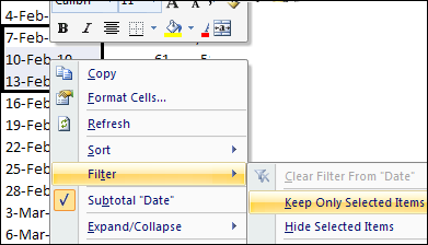
If you’re working with an Excel pivot table, you might want to temporarily hide one or more of the items in a Row field or Column field. To do that, you probably click the drop down arrow for the Row or Column Labels, then remove the check mark for items you want to remove.
As the storm clouds rolled in yesterday afternoon, I tweeted about saving my Excel files more frequently, as a safety precaution.
There were a couple of responses, asking why I didn’t use Excel’s AutoSave feature, and Jon Peltier reminded me to use AutoSafe — Jan Karel Pieterse’s free add-in.
AutoSave Add-In
I mentioned AutoSafe in my Excel New Year’s Resolutions 2010 blog post, oh so long ago. Of course, I’ve kept all my resolutions — how about you?
Installing AutoSafe
Even though I’m a creature of habit, and like to manually save my files, or click my Backup macro button, I decide to install AutoSafe. Good timing too, since Jan Karel uploaded a new version on June 1st.
While downloading AutoSafe, I also grabbed a copy of the companion add-in, AutoSafe VBE. It backs up your Excel code, so that should also be handy to have.
I unzipped the download file, and double-clicked on the setup.exe file. The installation wizard warned me to close my Excel files, and the installation was quick and easy.
Setting up AutoSafe
When I opened Excel 2007, the add-ins appeared on the Ribbon’s Add-ins tab. Click the AutoSafe command to open a dialog box where you can change the settings.
Choose the folder where you want the backup files stored, and the interval for the saves, and select any other options you want. To check for new versions, click the Update button.
Autosafe Settings Dialog Box
Setting Up AutoSafe VBE
The settings for AutoSafe VBE are similar, and you can also set the number of generations that you want to save. The CleanUp button clears out all the old files for you.
Old Habits
It’s hard to break old habits, so I’ll probably continue to press Ctrl + S every few minutes, to save my work. It won’t hurt to have some extra help though, especially when working on code revisions. Thanks Jan Karel, for this wonderful free add-in.
And I don’t know why, but typing “old habits” reminded me of The Flying Nun, starring Sally Field. Ah yes, the golden age of television! Here’s the opening segment, for those who don’t know what the heck I’m talking about.
Have you installed Office 2010 yet? Would you like to win a copy, along with a couple of other great prizes? [for USA residents only]
In this short video, Microsoft employees and customers talk about the benefits of Excel 2010, both for the users and the IT department. Watch carefully — there will be a test later!
VIDEO IS NO LONGER AVAILABLE
The Future of Productivity Giveaway
The nice people at Ignite Social Media invited me to participate in a giveaway [for USA residents only], as part of the Office 2010 launch. No free stuff for me, but one of you can win a cool prize package. Yes, there’s probably a better adjective than “cool” — at least I didn’t say “groovy”. 😉
The Prize Package
one (1) copy of Microsoft Office 2010: Home and Business
a Flip Ultra HD Camcorder
a Seagate FreeAgent Desk Hard Drive (1 TB)
Here’s a picture of the prize package, obviously not shown to scale! The pictures are from the Microsoft Store site, so the actual prizes might look different. Based on the prices shown in the Microsoft Store, the prize value is approximately $589 USD.
How to Enter
The giveaway is a scavenger hunt, so you’ll have to watch the video (at the top of this post) to find an answer to this question:
How does Excel 2010 make data analysis and reporting better/easier?
Add a comment below, with a unique, relevant answer to the question shown above. (Don’t just copy someone else’s comment!)
The Giveaway Rules
You must be a resident of the Unites States of America.
The entry deadline is 12:00 noon (Eastern time zone) on Tuesday, June 8th, 2010.
One entry per person – any additional entries will be deleted from the draw
A random draw will select the winner from all valid entries.
Winner will be notified by email, so please provide a valid email address. This will not be publicly visible, but will be shared with the contest organizers at Ignite Social Media, so they can contact the winner to arrange delivery.
The winner will be announced in this blog on Wednesday, June 9th.
More Future of Productivity Events
This widget has more videos, and you can click to learn more about the Future of Productivity launch.
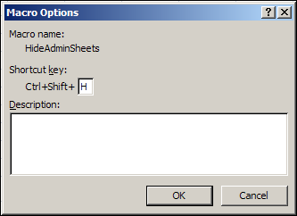
In a workbook, you might have some sheets that everyone uses, and other sheets that only one or two people need to use, for Admin functions. For example, the workbook shown below has a data entry sheet for orders, and two Admin sheets — one for lists and one for workbook options.
Occasionally, I get calls from clients who don’t understand why their Excel file isn’t working. They’re clicking buttons, or selecting from drop down lists, but none of the usual magic is happening. Is the file broken?
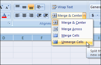
I saw this on Twitter yesterday: Wanted “Break Apart all merged cells in entire spreadsheet” button. If you’ve done much work in Excel, you’ve probably encountered problems that are the result of merged cells on a worksheet.
Merging cells can seem like a good idea at the time, but can interfere with sorting and filtering, and other things that make an Excel workbook useful. Here’s how you can unmerge Excel cells.
In the example shown below, orders with a quantity greater than 50 are highlighted with green fill colour.
cells highlighted with green fill colour
Conditional Formatting Rule
This was the result of simple conditional formatting, based on the cell value.
Sometimes though, the conditional formatting can be distracting, and there’s no built in way to temporarily remove it.
Edit Formatting Rule dialog box
Create an On/Off Switch
Instead of removing the conditional formatting, you could add an On/Off switch to your worksheet. Then, adjust the rules, so you only show the conditional formatting when the switch is on.
In the screenshot below, there’s a cell named CondF_Show, and it has a data validation drop down for Yes and No.
cell named CondF_Show
Change Conditional Formatting Rule
I changed the conditional formatting to a formula that checks both the Quantity cell value, and the value in the CondF_Show cell.
Change Conditional Formatting Rule
On/Off Switch Set to No
After you revise the rule, when the CondF_Show cell is changed to No, the conditional formatting is temporarily hidden.
On/Off Switch Set to No
More Conditional Formatting Info
For more Conditional Formatting rules and advanced examples that use a formula, go to the Conditional Formatting Examples page on my Contextures site.
And here are a few more pages on my site, where you can learn more about Excel Conditional Formatting:
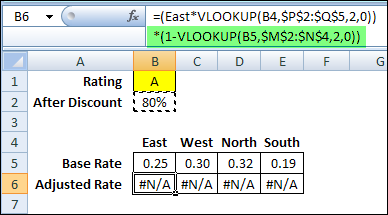
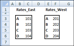
You can use the VLOOKUP function to find data in a lookup table, based on a specific value. If you enter a product number in an order form, you can use a VLOOKUP formula to find the matching product name or price. See how to use Excel VLOOKUP in different ranges.
NOTE: The examples below use VLOOKUP to get the value from the correct table. You could do a similar lookup with the INDEX and MATCH functions.