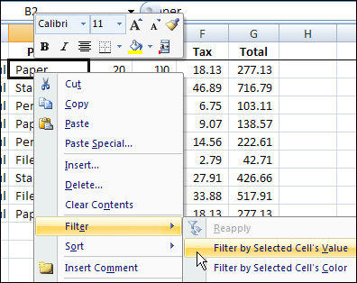
Last month you saw a quick way to filter for the selected item in a pivot table, and today you’ll see a similar technique for a worksheet list in Excel 2007.
Tip: For the Excel 2003 quick filter instructions see AutoFilter By Selection in Excel
Excel tips and tutorials

Last month you saw a quick way to filter for the selected item in a pivot table, and today you’ll see a similar technique for a worksheet list in Excel 2007.
Tip: For the Excel 2003 quick filter instructions see AutoFilter By Selection in Excel
Yesterday was Canada Day, and Sunday is the July 4th celebration in the USA, so your brain might be in holiday mode today.
Instead of a long, complicated blog post, here are a few quick Excel tips, in very, very, short videos. The longest one is 15 seconds!
You don’t have to live with the default number of sheets in a new Excel file. Instead of having 3 blank sheets in each new workbook, you can reduce the number, or increase it.
There are many more Workbook Tips on my Contextures site.
You can add or remove the features on the Excel 2007 Status Bar. For example, add new summary functions in the AutoCalc section, or show the status of special keys, such as Caps Lock or Num Lock.
There are many more Status Bar Tips on my Contextures website. For example, use the statistics section to help with formula troubleshooting.
If you want to be able to see the top few rows of a worksheet, even if you scroll down, you can freeze them.
There are many more Freeze Panes Tips on my Contextures site.
If your brain can absorb a few more quick tips, check out the Excel Quick Tips Videos on the Contextures website. Happy Holidays!
_____________
In the past, I highly recommended the Excel newsgroups as a place to go for help. However, earlier this month, Microsoft shut down their newsgroup servers, where thousands of people every month had gone to post their Excel questions, and the Excel newsgroups disappeared.
[Updated 2020-12-09]
Continue reading “Excel Newsgroups Disappeared-Find Excel Help Resources”
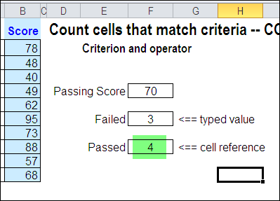
One of the tasks you have to do quite often in Excel is to count things. Here’s how to count cells greater than set amount with Excel COUNTIF function.
Continue reading “Count Cells Greater Than Set Amount With Excel COUNTIF Function”
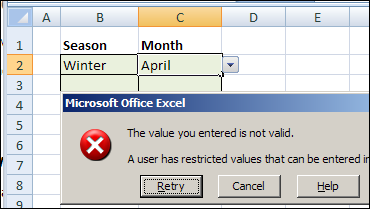
Why are invalid entries allowed in Data Validation sometimes?
Have you ever set up a data validation drop down list, so you can select valid items from a drop down list. But instead, Excel allows people to type anything they want into that cell?
See why that happens, and how you can prevent the invalid entry problem.
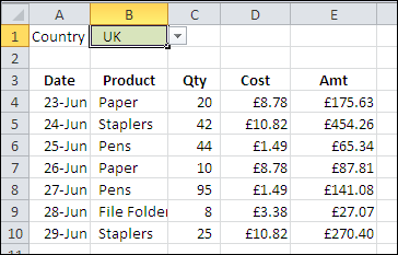
If you sell products in several countries, you might want to show the prices in different currencies.
In Excel 2010 and later, you can use conditional formatting for currency symbol changes.
See how to use those settings, you can change the number format based on a cell’s value, to show a specific currency for the country that’s selected.
There are written steps and a video below
Continue reading “Conditional Formatting for Currency Symbol”
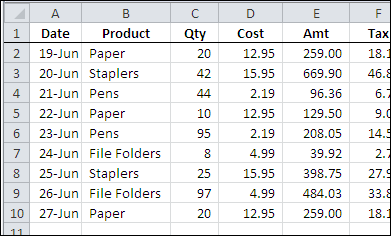
It’s finally summer, and you need to stay cool, even when you’re using Excel. Here’s an energy-efficient and fast way to find and delete Excel rows. You can select several rows that contain similar data, and delete them all at the same time.
If you add pictures to an Excel workbook, the file size can increase pretty quickly. And if you’re updating the pictures occasionally, perhaps for a product catalogue, you’d have to remember to update all the Excel files that have those pictures.
Instead of adding the pictures to the Excel file, Ron Coderre has created a sample workbook that displays pictures from a network file folder or even a web folder.
You can distribute Excel workbooks with links to the picture files, and that will mean smaller files, and easier updates
In the Excel workbook where you want the pictures, create a list of picture names, with file path and file names in the adjacent column. In the example shown below, two files are in the C drive, and one is on the internet.

In Ron’s sample file, the list of picture file names is in a range named LU_DisplayName. The picture names and file locations are in a range named LU_Name_FileLoc_XRef.
Using data validation, Ron created a drop down list where users can select one of the picture file names. The data validation cell is named rngDisplayName.

A VLOOKUP formula returns the location of the selected picture file, in a cell named rngFileLocation.
![]()
The selected picture is displayed in a range named rngPicDisplayCells.

To make the selected picture show on the worksheet, Ron added some event code to the worksheet. When the data validation cells changes, the code runs, and shows the selected picture file.

In Ron’s sample file, you can view the detailed instructions for setting up the workbook and displaying the pictures.
He describes the data validation setup, the named range formulas and the VBA code to make everything work.
To see how the picture display works, you can download Ron’s sample file from the Contextures website.
In the “Charts and Graphs” section, look for “RCH0002 – Insert Pictures from Folder”.
The file contains macros, so you’ll have to enable them to test the file. There are two versions of the file — one for Excel 2007 an done for earlier versions. Both sample files are zipped.
__________________
This offer has expired.
For the latest Excel courses, Excel books and Excel tools, go to the Debra’s Excel Picks page, on my Contextures website

____________
How can you get missing data to show up in your Excel pivot table, showing a count of zero? AlexJ encountered this problem recently, and sent me his solution, to share with you.