
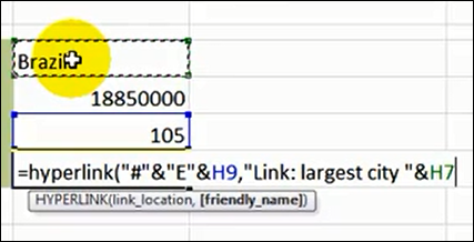
Last week, I heard from Kevin Lehrbass, who runs the My Spreadsheet Lab website. Kevin has posted an Excel video on YouTube, that shows how you can make a dynamic hyperlink, using array formulas.
Category: Excel Formulas
Excel Average Based on Multiple Criteria
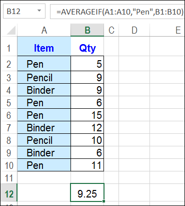
In Excel, you can use the SUMIF and COUNTIF functions, to sum and count values, based on criteria. Did you know that you can also calculate an Excel average, based on multiple criteria?
Create Amazon Affiliate Links in Excel
This week, Dick Kusleika posted his Amazon Linkerator – an Excel file lets you create links to Amazon products.
First, you find a product on Amazon, and copy its web page URL. Then, open the form, enter a product code and description, and it creates a link for you.

It’s very fancy, and you can download the sample file, to try it for yourself. It uses an Excel UserForm, and you can modify the code to add your own information.
Jimmy Pena has an Amazon Link Builder too, and you can see the details here: Amazon Link Builder
Low Tech Amazon Link Builder
I build Amazon links too, and you can see lots of them on my Excel Book List page.
To create my links, I use worksheet formulas, instead of a fancy UserForm. If you like things simple, you can try this method.
You enter the product code and product title, and then copy the link or the HTML code, and paste it into your blog post or web page.
WARNING: Check the latest information on the Amazon website, to be sure that these short links are still permitted. Their policies can change at any time.

How It Works
First, a link is created in cell B5, from the Amazon URL, the product code (ASIN) and the Tracking ID.
=https://amzn.com/ & ProdCode & “?tag=” &TrackID
Note: Cell B3 is formatted as Text, because some codes start with a zero, and you don’t want Excel to remove those.

Then, that link is used in the to create the HTML code in cell B7.
The four HTML cells have snippets of text that are required for building the HTML code. The formula in cell B7 combines the product title and the link, with four snippets of text.
=HTML_01 & ProdTitle & HTML_02 & ProdLink
& HTML_03 & ProdTitle & HTML_04
Download the Sample File
To test the Amazon link formulas, you can download my sample file, from the Excel Sample Files page on my Contextures website. In the Functions section, look for FN0025 – Build Amazon Affiliate Links
____________________
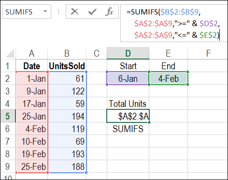
Sum For a Date Range in Excel
First, some news about the upcoming Office 365 launch, and then a tip on how to sum for a date range in Excel.
Round to a Nickel in Excel
If you’ve been following the Canadian news (and who isn’t?), you know that the penny has been eliminated from circulation. To honour the occasion, Google made a special doodle for google.ca on February 4, 2013.

Rounding Guidelines
If you’re shopping with cash now, the final amount will be rounded up or down, to the nearest nickel. There are guidelines posted on the Royal Canadian Mint’s website: Eliminating the Penny: Rounding [article no longer available]

Rounding to the Nearest Cent
As an example, the Mint’s website shows the purchase of coffee and a sandwich, with tax, for a grand total of $4.86.
The tax department says to round the tax to the nearest cent, so you can use Excel’s ROUND function for to calculate the HST. Just multiply the subtotal by the tax rate, and round to 2 decimal places. Here is the formula in cell B6:
=ROUND(B5*D6,2)

Rounding to the Nearest Nickel
With the HST, the grand total for the lunch is $4.86. We don’t have pennies now, so the cash payment will be rounded to the nearest nickel. Excel’s ROUND function can’t help with that.
Fortunately, there is another rounding function – MROUND – that can round to a specified amount.
- The MROUND function has two arguments – the number, and the multiple.
In this example, we want to round the grand total, which is in cell B7. We’ll enter the multiple in cell B9, to show how the cash payment was rounded.
Here is the cash payment rounding formula in cell B10:
=MROUND($B$7,$B$9)

- Note: For Excel 2003 and older, the MROUND function is available after you load the Analysis Toolpak add-in.
Test the MROUND Formula
A nickel is worth 5 cents, so what happens if you enter a 5 in cell B9, to use as the multiple?

Oops! That rounds the amount to 5 dollars, instead of the nearest nickel.
Change the amount in cell B9 to 0.05, which is the way that you’d enter a nickel amount in a worksheet.

Perfect! With the MROUND function, and a multiple of 0.05, you can round those sales totals to the nearest nickel.
____________________
Round to a Nickel in Excel

________________
New ISFORMULA Function Excel 2013
Last week, we took a look at the new FORMULATEXT function in Excel 2013. Another one of the new features in Excel 2013 is the ISFORMULA function.
Finally, there’s a way to identify cells that contain a formula, without creating a User Defined Function to do the job.

TYPE Function Problems
The TYPE function was originally designed to show what a cell contained, such as text or a formula. It returns a number to show the type for a cell’s contents, or a formula’s result.
Here’s the list of results, and the data types:

In a few versions of Excel, the Help files incorrectly reported that a formula would return 8 with the TYPE function, but unfortunately, that’s not the case.
Check for a Formula
With the new ISFORMULA function, you can test a cell, to see if it contains a formula.
In the screenshot below, the following formula is entered in cell B4, and copied across to cell D4:
- =ISFORMULA(B2)

The result in cells B4 and C4 is FALSE, because cells B2 and C2 have numbers typed in them.
The result in D4 is TRUE, because cell D2 contains a formula.
Highlight Cells With Formulas
You can use the ISFORMULA function with conditional formatting, to highlight cells that contain formulas.
In the screen shot below, cells in column C have a formula, and they are shaded grey.

For the details on how to apply this type of conditional formatting, and for more information on the ISFORMULA function, you can visit my Contextures website: Excel ISFORMULA FUNCTION
_____________________
Show Formulas with FORMULATEXT Excel 2013
There is a new function in Excel 2013 – FORMULATEXT – that lets you show the text from a cell’s formula.
In the screen shot below, cell C2 contains the formula:
=FORMULATEXT(B2)

Matches Formula Bar
The FORMULATEXT result shows the formula that’s in cell B2, just as if you had clicked on cell B2 and looked in the formula bar.

Use FORMULATEXT for Troubleshooting
You can use FORMULATEXT for auditing or troubleshooting a worksheet. For example, combine FORMULATEXT with the INDIRECT function, to check the formula in any cell.
In the screenshot below, a cell address (B2) is entered in cell B4, and the FORMULATEXT result shows the formula from cell B2.
=FORMULATEXT(INDIRECT(B4))

More on FORMULATEXT
For more FORMULATEXT information and examples, please visit my Contextures website. You can read the details there, and download the sample file: Excel FORMULATEXT Function
Video: Excel FORMULATEXT Function
To see the steps for creating a FORMULATEXT function, and a few examples, you can watch this short video tutorial.
______________
Choose Report Dates With Excel Scroll Bar
This week, I’ve been working on some dashboards, and want to make it easy for people to select a date range for the report.
I experimented with drop down lists and slicers, and finally settled on a good old-fashioned scroll bar. You can click or drag the scroll bar to select an end date, and see three months of sales data, and the total.
Note: The technique does NOT require programming and is fairly easy to set up.

Scroll Bar Select the End Date
The scroll bar on the Summary sheet is linked to a named cell on another sheet, and that number is used in an INDEX / MATCH formula, to calculate the end date.
The date headings have formulas that show the selected end date, and the two prior months.

Get Data From a Pivot Table
The sales data is summarized in a pivot table, by report month, and region.

GetPivotData Formula
The summary table uses the GETPIVOTDATA function to pull the correct data, based on the region name and the date.
The IFERROR function returns a zero, if the data isn’t found in the pivot table.

Download the Sample File
To download the sample file, and see the written instructions, please visit my Contextures web site: Select Date with Excel Scroll Bar
__________________
DSUM and Excel Tables: Sum With Multiple Criteria
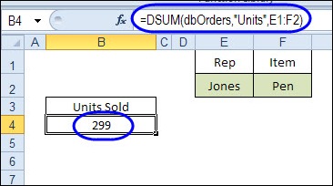
If you need to get a total in Excel, based on criteria, there are a few different ways that you could do it. Today, we’ll take a look at how DSUM and Excel Tables sum with multiple criteria.
Continue reading “DSUM and Excel Tables: Sum With Multiple Criteria”
Product Code Lookup in Date Range
Steve emailed me this week, to see if I could help with a lookup problem. He needed to find a discount rate in a lookup table, based on a product code and a date range.
Here is how I solved the problem in Excel 2010 (using fake data), and please let me know if you have a different solution.
Product Pricing Sheet
On a separate sheet, there is a list of products and their prices. This list is formatted as a named Excel table – tblProducts. The two columns in the table are also named – ProdCodeList and ProdPriceList.

Promotions Sheet
On another sheet, there is a list of the promotions that have been offered. This table is named tblPromotions, and each column is also named. We’ll use those names in the formulas.
In this table, I added an ID column at the left, and entered a unique number in each row. The existing Promo Code column has text entries, and for my solution I needed a numeric ID in each row.

Orders Worksheet
On the Orders sheet, a record is created for each new order, with the order date, product code and quantity entered. This table is named tblOrders.
NOTE: Because the formulas are being created in a table, you’ll see column references, like [@Qty], instead of cell references.
You can use an INDEX / MATCH formula to get the product price, based on the product code:
=INDEX(ProdPriceList,MATCH([@[Prod Code]],ProdCodeList,0))
For the subtotal, multiply the product price by the quantity
=[@Qty]*[@[Unit Price]]

Find the Applicable Promotion
The next step is to check the promotions table, to see if there was a promotion for the selected product, when the order was placed.
To do that, I used a SUMIFS formula (NOTE: only available in Excel 2007 and later versions):
=SUMIFS(PromoIDList,
PromoStartList,"<=" & [@[Order Date]],
PromoEndList,">=" & [@[Order Date]],
PromoProdList,[@[Prod Code]])
This formula returns a number from the PromoID column, if a promotion is found that matches the criteria:
- Promo start date is on or before the order date
- Promo end date is on or after the order date
- Promo product code matches the order product code
If no matching promotion is found, the sum will be zero. Otherwise, the Promo ID will be the sum.
NOTE: This solution depends on there not being any overlaps in dates for a product promotion. Each promotion ends before another one for the same product begins.

Find the Promo Code
Once the Promo ID has been found, the Promo Code can be looked up, using INDEX and MATCH, based on the Promo ID.
=IFERROR(INDEX(PromoCodeList,
MATCH([@[Promo ID]],PromoIDList,0)),"N/A")
This formula returns a promo code, if a promotion is found that matches the promo ID. If there is no match, the result is “N/A”.

Find the Promo Discount
The same type of INDEX and MATCH formula is used to find the discount rate, based on the Promo ID.
=IFERROR(INDEX(PromoDiscList,
MATCH([@[Promo ID]],PromoIDList,0)),0)
This formula returns a discount, if a promotion is found that matches the promo ID. If there is no match, the result is 0.

Calculate the Total
Finally, to calculate the total amount, we multiply the subtotal by 100% minus the discount rate.
=[@Subtotal]*(1-[@Disc])

Download the Sample File
To download the sample file, please visit my Contextures website: Excel Sample Files – Functions Section.
Look for FN0023 – Product Code Lookup in Date Range
_____________________