If you have a list of names in Excel, with first and last names separated by a comma, you can use an Excel feature to split first and last names into separate columns.
It’s Friday, and things are slow at the office. To liven things up, you could create bingo cards in Excel, and organize a game during the lunch hour.
In this example, there are three cards, each with a set of random numbers. You’ll need one of those numbered ball popper machines though, or create a number selector in Excel. Continue reading “Create Bingo Cards in Excel”
One of my clients coached his women’s hockey team to a provincial championship last weekend (and this is the medal they were awarded). Congratulations to him and the team!
I don’t think he used Excel in planning his coaching strategy, but I’m sure Excel has other uses in sports.
Assign Baseball Players
For example, one of the Excel sample files on my website lets you assign baseball players for each inning. After you assign a player in an inning, that player’s name is removed from the drop down list for the inning.
You can’t accidentally assign the same player twice. You can download the zipped file here: DataValPlayerInnings.zip 3kb
The other version has a UserForm in which to enter the tee off data: GolfTeeOffForm.zip 16 kb
Analyze Walking Targets
In another sample file, you can record the number of steps you’ve walked each day, and formulas will calculate if you’ve reached the thresholds that you’ve set.
It keeps track of your streaks, such as the greatest number of consecutive days that you’ve achieved each target.
You could adapt this to other sports or personal goals.
Sadly, I don’t have any hockey sample files, but I found a Hockey Analytics site that has Excel and pdf files you can download.
For example, there are several Excel files with calculations for Individual Player Contributions, and a few with Personal Goals Against Averages.
If you like statistics and hockey, you’re sure to find something of interest. But remember, as the Hockey Analytics site points out:
Baseball is a game of a limited number of states…It can be modeled accurately in discrete steps…This ain’t the case with hockey. Hockey is fluid and can only be modeled approximately…Hockey statistics are terribly incomplete.
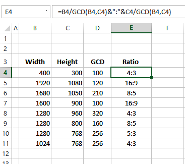
In Excel, if you divide 2 by 8, the result is 0.25. If you format the cell as a fraction, the cell might show 1/4 as the result. But how can you calculate a ratio in Excel? See the written steps and video below.
Recently, I read a business article that said you should “become a Roman” to succeed in business. By that, the author meant, “be disciplined and willing to keep fighting”.
Excel ROMAN Function
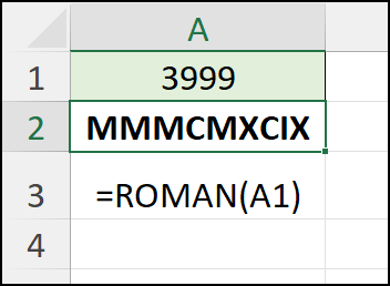
Maybe that’s why we have the Excel ROMAN function! It will quickly convert a worksheet number into Roman numerals.
That frees up our time, so we can “keep fighting” to fix other problems in our Excel files.
In the sections below, I’ll show you how the ROMAN function works. And I found a couple of fun facts about ROMAN, that might impress your friends and co-workers. (Or not!)
Excel ROMAN Function Syntax
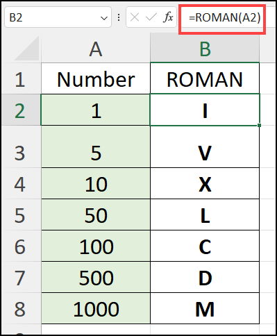
Here are the two arguments in the ROMAN function:
number: an Arabic number, between 0 and 3999, that you want to convert to Roman numerals.
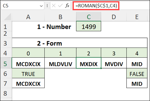
form: (optional) the type of conciseness that you want to display.
This week I’ve been working on date formulas, from very simple ones, to complex formulas that calculate workdays per month, based on start and end dates that can span several months.
Extract Information from a Date
Many times I need to pull a bit of information from a date, such as the year, month or weekday.
In the section below, I’ve listed the sample Excel formulas I would use, to calculate specific dates in Excel.
For all formulas, the date — December 29, 2008 — is in cell A2.
Date Calculation Formulas
Date Calculation Formulas
Here are the formulas to extract information from a date in cell A2.
To Calculate
The Formula
The Result
Year
=YEAR(A2)
2008
Month Number
=MONTH(A2)
12
Month Name (short)
=TEXT(A2,”mmm”)
Dec
Month Name (long)
=TEXT(A2,”mmmm”)
December
Day of the month
=DAY(A2)
29
Weekday Number
=WEEKDAY(A2,1)
2
Weekday Name (short)
=TEXT(A2,”ddd”)
Mon
Weekday Name (long)
=TEXT(A2,”dddd”)
Monday
Year Month
=TEXT(A2,”yyyy mm”)
2008 12
Using Calculated Dates in Pivot Table
If I plan to create a pivot table from data that contains a date field, I usually calculate the year and month in the source data.
Then I can add those fields to the pivot table, instead of the individual dates.
Yes, the pivot table could automatically group the individual dates by year and month, but that can limit other functions in the pivot table.
For example:
if two pivot tables are based on the same data, grouping one pivot table by month would cause the other pivot table to also be grouped by month.
if a field is grouped, you cannot add calculated items to the pivot table
pivot table error message – cannot add a calculated item
Video: Pivot Table Grouping Tips
This video shows how to group pivot table dates by month and years, and how to group text items manually.
There are examples for grouping dates, number and text fields. You’ll also see solutions for fixing pivot table grouping problems, such as the error message, “Cannot group that selection”
Excel formula to calculate 4th Thursday in November
Video: Find Nth Weekday
[Update} I made this video in 2022, and the formula uses the WORKDAY.INTL function, which is available in Excel 2010 or later
This video shows how to find the Nth weekday in a specific month and year, by using the WORKDAY.INTL function in an Excel formula.This function is available in Excel 2010 or later.
To calculate the date in earlier versions of Excel, use one of the WEEKDAY formulas on the Find Nth Weekday in Month page, on my Contextures site.
Last weekend I set up a little spreadsheet in Excel to compare the cost of a trip in a rented RV versus a small car. The only gas consumption numbers I could find for the RV were in miles per gallon.
Convert to Metric
Since we use the metric system here in Canada, I needed to convert everything to kilometres and litres.
Fortunately, Excel has a CONVERT worksheet function that makes the conversion easy.
The only tricky part is remembering the codes for each type of unit. Most are intuitive, such as ft for foot and g for gram, but a few aren’t, like lbm for pound mass.
Convert Litres to Gallons
To calculate how many litres are in a gallon, I used the formula:
=CONVERT(1, “gal”,”l”)
In the formula, gal is the code for gallon, and l (lower case L) is the code for litre.
And yes, it’s way more expensive to make the trip in an RV.