Let it snow! One of the advantages of working from home in Canada, is that you don’t have to go out in rush hour, on snowy days. I can sit in my office, basking in the glow of the computer monitor, mesmerized by the flickering of the modem lights.
But eventually I’ll have to go out to do some shovelling, in the sub-zero temperatures. Later, while thawing out, I’ll create an Excel file, to track the miserable temperature and snowfall accumulation.
A Matter of Degree
 We record our temperatures in Celsius, while our neighbours in the USA use a Fahrenheit scale. So, while I’m shivering on a -10°C day, it seems much warmer across the lake, where it’s a balmy 8°F.
I’m sure there are good reasons why the USA didn’t switch to the metric system when Canada did, but for now, we can use Excel to convert the temperatures.
Use Arithmetic
Maybe the temperature in the USA really isn’t as warm as it seems.
To convert the temperature from Fahrenheit to Celsius , you can use this formula:
- °C = (°F – 32) x 5/9
If the Fahrenheit temperature is in cell B2, put this formula in cell C2:
- =(B2 – 32) * 5/9
When I convert that balmy 8°F, it makes me feel better – it’s actually colder there, at -13°C.
Let Excel Convert It
That formula isn’t too difficult, but it might be hard to remember if your brain is affected by the cold weather. An easier way to convert the temperature is to use Excel’s CONVERT function.
- Note: If you’re using Excel 2003, or an earlier version, you’ll need to install the Analysis ToolPak to use the CONVERT function.
Excel CONVERT Function
With the CONVERT function, you refer to the cell that contains the amount that you want to convert. Then you enter the original unit of measurement, and then the new unit of measurement.
We want to convert the value in cell B2, from Celsius (“C”) to Fahrenheit (“F”).
- =CONVERT(B2,”C”,”F”)
Later, I can use CONVERT to see how many inches of snow we got, when the weather channel reports the snowfall in centimetres.
Excel Help for CONVERT Units
If you aren’t sure what code to use for each unit of measurement, you can check the list in Excel’s help for the CONVERT function.

Now I have to go and figure out how many glasses of wine are in that 750 ml bottle. I think the answer might be – not enough!

___________