
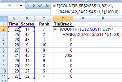
To do some research on sorting, I hauled one of the big, dusty Excel books off my shelf, to see if there were any scintillating sorting secrets to uncover. Under Sorting, I saw “rank calculations” so I turned to that page, to see what it said about calculating rank in Excel.
Category: Excel Formulas
Count Cells With Specific Text in Excel
While working on a client’s sales plan last week, I had to count the orders for a couple of specific customers. This tutorial shows how to count cells with specific text in Excel.
Plan Your Party Seating with Excel
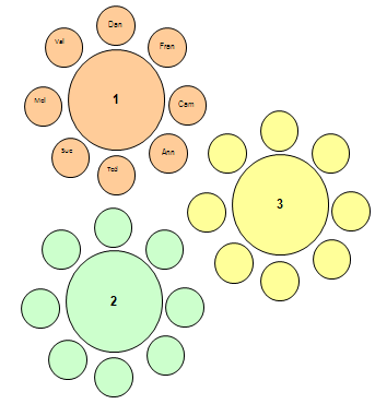
If you’re having a party this weekend, you can plan your party seating with Excel. Get this sample Excel seating workbook, enter the guest names on the Lists sheet, then fill the tables by selecting names from data validation drop down lists. After you’ve assigned a guest to a table, that guest’s name disappears from the drop down lists, so you can’t accidentally assign a guest to two different seats.
NOTE: There is a newer seating plan here: Excel Seating Plan with Charts
Clean Excel Data With TRIM and SUBSTITUTE
You have two Excel lists, and you’re trying to find the items that are in both lists. You know there are matching items, but if your VLOOKUP formulas can’t find any matches, you might need to clean Excel data with TRIM and SUBSTITUTE.
Continue reading “Clean Excel Data With TRIM and SUBSTITUTE”
Excel Price List With VLOOKUP and MATCH Function
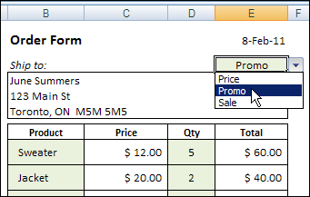
You can create order forms and price lists in Excel, and automatically show a price when a product is selected in the order form. But what happens if you want to give some customers special pricing, or offer sales pricing occasionally? Here’s how to customize your Excel price list with VLOOKUP and MATCH.
Continue reading “Excel Price List With VLOOKUP and MATCH Function”
Calculating Ages in Excel
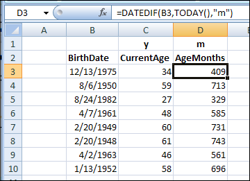
Can you remember how old you are? Or are you like me, and have to ask, “What year is it?” and then subtract your birth year? Or do you like calculating ages in Excel — let it do the arithmetic for you!
Excel OFFSET Function-Fish for Data
That’s my dad in the picture below, proudly holding the catch of the day. He tried to teach me how to fish, but without much success. (Worms…ewwww.)

Fishing with OFFSET Function
This week someone asked me to explain the Excel OFFSET function, saying “Please teach me to fish.” That’s when it struck me that using OFFSET is similar to fishing.
- When you’re fishing, you can dip into a pond with a bamboo pole and a small hook, or head out to sea, and cast a large net. Or you can fish the way we do in Canada, through a small hole in the ice, but that’s another story. (There’s a video at the end of this article.)
- With the Excel OFFSET function, you can pull data from a single cell nearby, or a large range of cells off in the distance.
The OFFSET function is useful when you want to make the data selection adjustable.
For example, if a February date is entered in cell A2, you can sum the February expense column. If a March date is entered, sum the March expenses instead.
Your Fishing Equipment
To make the OFFSET function work, you’ll tell it 3 things:
- The starting point
- Where to go from there
- How big a range to capture (optional)
The OFFSET syntax is: OFFSET(reference,rows,cols,height,width)
- The reference is the starting point.
- The rows and cols tell OFFSET where to go from the starting point. It can go up or down a specific number of rows, and left or right a specific number of columns.
- The height and width set the size of the range. It can be as small as 1 row and 1 column (a single cell) or much bigger.
For example, this OFFSET formula would return the January total, in cell B6:
=OFFSET(A1,5,1,1,1)
- The starting reference is cell A1.
- From there, it goes down 5 rows, and right one column, to cell B6.
- The selected range size is 1 row tall and 1 column wide.

Baiting the Hook
Instead of typing all the values in the formula, you can use one or more cell references, to make the OFFSET formula flexible. In this example, all the totals are in row 5, so that number won’t change.
However, the month number is typed in cell G1, so you could use that cell to set the number of columns to offset. Change the formula so G1 is the cols argument.
=OFFSET(A1,5,G1,1,1)

Now, if you change the month number to 3 in cell G1, the March total will be returned.
Casting the Net
Instead of pulling the result from a single cell, you could use OFFSET with the SUM function, to select a range with multiple cells, and calculate the total.
For example, this formula would calculate the total for the February expenses.
=SUM(OFFSET(A1,1,G1,4,1))
- The starting reference is cell A1.
- From there, it goes down 1 row, and right 2 columns, to cell C2.
- The selected range size is 4 rows tall and 1 column wide – C2:C5.

Other Fish to Fry
I like the OFFSET function, and use it to create dynamic ranges in some of my workbooks.
There are alternatives to using the Excel OFFSET function, such as the Excel INDEX Function.
There’s an interesting discussion of the merits of each function on Dick Kusleika’s Daily Dose of Excel Blog: New Year’s Resolution: No More Offset.
Ice Cold Fish
I’d rather stay inside and work on OFFSET formulas, but ice fishing is popular here in Canada. This video makes the sport look almost appealing.
_____________________
Does Excel Drive You to Drink?
After a long day of dealing with Excel formulas, pivot tables, and hidden Ribbon commands, you might be ready for an evening cocktail. Or six!
Newspaper Study
I found a link to this Canadian drinking study in the Toronto paper today, and it looks like we’re a nation of teetotalers. Is your country the same?
Apparently most Canadians don’t work with Excel, or perhaps they vent their frustrations on the hockey or curling rink at the end of the day.

The Excel Drink Calculator
To spare you the agony of checking your results in a hard-to-read green pie chart, I created an Excel version of the online drink calculator.

Use the Drink Calculator
In cells C3 to C9, enter your estimated number of drinks per day.
- The SUM Function in cell C10 calculates your total for the week.
Then, select Men or Women from the drop down list in cell C12.
- The VLOOKUP formula in cell C15 will compare your results to the rest of the men or women in Canada.
Hmmm…more than 85% – that can’t be good.
Time to move, I think. 😉 What country would you recommend?
Download the Excel Drink Calculator
If you’re brave enough to test your own results, you can download the Excel Drink Calculator. It’s in Excel 2007 format, with no macros.
Please do not operate heavy machinery, or leave a comment, if you have been drinking.
______
Elvis Sings Excel: A Little Less Concatenation
Last Friday, January 8th, would have been Elvis Presley’s 75th birthday. Sadly, he died in 1977, so he never had a chance to work with Microsoft Excel. Otherwise, he might have sung “A Little Less Concatenation”, instead of “A Little Less Conversation.”
Continue reading “Elvis Sings Excel: A Little Less Concatenation”
Create Excel Grand Totals With One Click
I hope you had a wonderful Christmas, and with any luck, you’re taking this entire week off.
You might still be full of turkey and eggnog, so I’ll just give you a quick and easy Excel tip today – something that’s easy to digest.
Create Quick Excel Grand Totals
Instead of entering each SUM function individually, you can use the AutoSum feature to create all the grand totals with one click.
Here are the simple steps to follow:
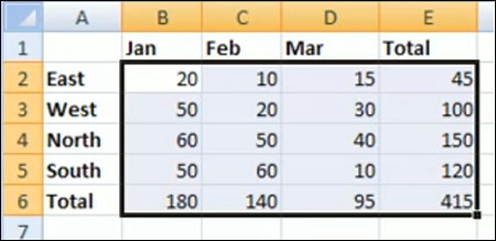
First, select all the cells with numbers, and the blank cells below and to the right, of those cells, where you want the grand totals
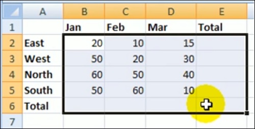
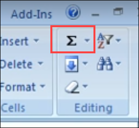
Use the AutoSum Button
Next, go to the Excel Ribbon, and click the Home tab
At the right end of the Home tab, in the Editing group, click the AutoSum button, to insert the Grand totals.
Grand Totals in Blank Cells
On the worksheet, the SUM function is added to each grand total cell, to sum the cells above, or to the left.
Watch the Video
To see me create Grand Totals in Excel with one click on the AutoSum button, you can watch this 12-second Excel video.
P.S.: For more Excel SUM tips visit my Contextures Excel SUM Functions page.