This week, I’ve been working in an Excel 2007 file that has several named Excel Tables. After adding a column in one table, I copied the entire worksheet column.
Next, I tried to paste it into another worksheet, where there was a similar table.
That didn’t go too well. After a few minutes of staring at the hourglass, I gave up, and closed Excel in the Task Manager.
Today, I tried to repeat the column copy and paste, forgetting about the previous problem.
Sure enough, Excel crashed again. Well, technically, I guess it’s a hang, rather than a crash, but it’s still annoying.
A Smaller Named Excel Table
In a smaller workbook, with smaller tables, the copy eventually completed, but with strange results. There was a strange message in the Status Bar.
Eventually, the copy completed, but instead of the ten rows from the original table, the paste filled the entire column, so the named Excel Table ended in the last row.
Successful Copy and Paste
Instead of copying and pasting the entire column, you can copy and paste the named Excel table column.
To select the table column, click, the top of the table heading cell, instead of the column heading button.
Then, to paste into the other table, right-click the heading cell, and paste.
Or you can copy the cells, and paste them, instead of copying and pasting the column.
How Do You Crash Excel?
Enough about my problems! What’s your favourite way to crash/hang Excel?
________________
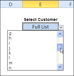
On Monday, AlexJ showed us how to create a short or long drop down list in Excel. With his technique, users can see just the top customers, or all customers.
That technique didn’t require macros — it was driven by a formula in the data validation source.
Long or Short List Macro
Today, Alex shares an automated version of the short or long data validation list technique. Starting in the next section, you can read his description of how this version works.
You can download the zipped Dynamic Data Validation Sample File from the Contextures website. The file contains macros, so enable them to use the dynamic drop down list.
Dynamic Data Validation Lists
For an Excel utility running at our office, users are required to enter a project number using a drop down list. There are thousands of these records in the data set, selecting from hundreds of project numbers. This means that the drop-down list is long, and therefore not very useful.
To address this, we determined that the user would usually select from a short list of active projects, but would also need to select from a long list of all projects or old projects.
Use a Single Drop Down
There are a number of techniques using dependent data validation in Excel, but these usually require two selection boxes, we wanted to do this with only a single drop down selection.
The technique presented allows the user to select from a default list of entries, or select a different list.
How It Works
The two lists are named — rng.DD1 for the new projects, and rng.DD2 for the full project list. The first cell in each list is a formula, that refers to the other list.
=”>> GOTO ” & $J$3
The cell with the drop down list is named rng.DD_Select.
Calculate Which List Selected
The result cell, $E$5, calculates which list has been selected:
=”rng.DD”&IF(rng.DD_Select=$J$3,2,1)
If the selected item matches the heading in cell J3, the result is rng.DD2, otherwise, the result is rng.DD1.
The Data Validation
The data entry cell has data validation configured for a list, and the following formula that refers to the result cell:
=INDIRECT($E$5)
If the result in cell $E$5 is rng.DD1, the new project list is shown.
The Programming
The data validation doesn’t require programming, but there is a small VBA routine triggered by the Change Event in cell B5. It tidies up the data entry cell, after a selection is made.
This routine will:
Clear any entries from the list where the user has selected “——–”, or a list header like “—– xxxx ——–”
Convert a selection like “>>>> GOTO NEW PROJECT LIST” to “NEW PROJECT LIST”
Excel Event Code
Here is the event code from the data entry sheet.
Private Sub Worksheet_Change(ByVal Target As Range)
Dim str As String
Dim strNew As String
Const strMatch As String = ">> GOTO "
If Target.Address = Me.Range("rng.DD_Select").Address Then
  str = Target.Value
  If str Like "-*" Then
    Target.ClearContents
  Else
    If str Like strMatch & "*" Then
      strNew = Right(str, Len(str) - Len(strMatch))
      Target.Value = strNew
    End If
  End If
End If
End Sub
You can make data entry easier in Excel, by create a drop down list with data validation. Sometimes those lists are so long, that they become a pain to use.
Here’s a technique from AlexJ, that lets users switch between a short or full Excel drop down list of customers.
Apparently there is a big football game this weekend in the USA. They’re using Excel for the game — XLV. That’s a really old version, but at least it has multiple sheets and VBA!
ROMAN Function
The officials probably used the Excel ROMAN function to figure out how to show the game number — 45:
=ROMAN(A2)
While you’re watching the game, you can use an Excel function to convert the field size from yards to metres. You’ll see that the American field is smaller than the Canadian field, no matter what measurement system you use!
Convert Metres to Yards
There is a CONVERT function in Excel, that you can use to convert measurements from one system to another.
=CONVERT(number,from_unit,to_unit)
For example, cell B3 has the length of a Canadian field in metres. In cell D3, the following formula converts that measurement to yards, and rounds the result:
=ROUND(CONVERT(B3,B$2,D$2),0)
Convert Metres to Yards
Unfortunately, the CONVERT function does not get you an extra point.
Other Differences
Besides the size of the fields, there are other key differences between Canadian and American football.
No stripes? Fewer players? More downs? You call that a game? 😉
Speaking of Excel 5.0
Do you remember when printed manuals came with the software? I still have my Excel 5.0 User Guide, so maybe I can read it while watching the big game!
There were tons of new features in that version, so there will be lots of interesting stuff to read.
This week, Carrie posted a comment on that article, and she wanted to adapt the bingo cards so they could be printed with Adobe InDesign. Instead of a square with 25 numbers, that program needs the 25 numbers in a single row.
Using the example in the screen shot above, the numbers in the first two rows would be arranged like this, followed by the numbers from the remaining rows:
Random Number Code
Jim Cone pitched in, and wrote some code to generate the random numbers in single rows, but it created some duplicates in the rows. Carrie didn’t want an uprising in the bingo hall, so we sent Jim away to try again. 😉
It didn’t take long for him to return with some code that worked correctly, so Carrie, and her Hummel figurine collecting friends, can safely play bingo this summer.
Whew! A bit later, Dick posted an update for Jim’s code. It’s shorter, and does the job very well.
Copy the Random Number Code
Thanks Jim and Dick! I’m sure Carrie appreciates the code, and maybe it will help a few other people.
To use this random number code, copy it to a regular code module in your workbook.
Then, go to a blank sheet, and run the SurelyYouCantBeSerious_R1 code.
Sub SurelyYouCantBeSerious_R1()
'Generates 800 sets of random Bingo numbers with no duplicates.
'Each row contains an individual set of Bingo numbers.
'Designed to be used with the "Adobe InDesign" application.
'Jim Cone - Portland, Oregon USA - February 02, 2011
'[email protected] - remove all "X"
'Edited by Dick dailydoseofexcel.com
On Error GoTo DontCallMeShirley
Dim arrList(1 To 800, 1 To 25) As Long
Dim j As Long
Dim R As Long
'B COLUMNS
'1 to 15 in the B column
Randomize
For R = 1 To 800
  For j = 1 To 5
    FillList arrList, j, R
  Next j
Next R
Range("A1:Y800").Value = arrList()
  Exit Sub
DontCallMeShirley:
  Beep
  Resume Next
End Sub
'==========
Sub FillList(ByRef arrList As Variant, lStart As Long, R As Long)
Dim j As Long
Dim C As Long
Dim N As Long
Dim arrCheck(1 To 75) As Long
j = 1
For C = lStart To 25 Step 5
  Do While j < 6
    'Int((High - Low + 1) * Rnd + Low)
    N = Int(Rnd * 15 + ((lStart - 1) * 15 + 1))
    If arrCheck(N) < 1 Then
      arrList(R, C) = N
      arrCheck(N) = N
      j = j + 1
      Exit Do
    End If
  Loop
Next C
End Sub
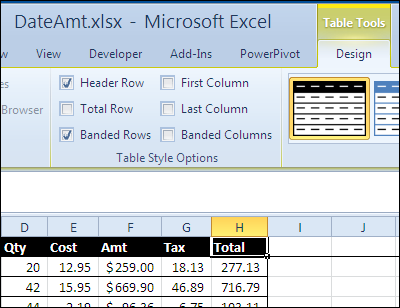
Now that the 30 Excel Functions in 30 Days challenge has ended, it’s time to look at a few other features. On the Contextures page on Facebook, Lee suggested AutoFilters as a topic for some February posts. Thanks Lee! Here’s how to turn off filters in Excel table headings.
Congratulations! You made it to the final day in the 30XL30D challenge. It’s been an long, and interesting, journey, and I hope you learned a few useful things about Excel functions along the way.
Tomorrow, I’ll do a wrap-up article, and let you know how the functions ranked in the pre-challenge voting, last month.
INDIRECT Function
For day 30, we’ll examine the INDIRECT function, which returns the reference specified by a text string.
This is one of the ways that you can create a dependent data validation drop down list, where, for example, the selection in the Country drop down controls the choices in the City drop down.
So, let’s take a look at the INDIRECT information and examples, and if you have other tips or examples, please share them in the comments.
Function 30: INDIRECT
The INDIRECT function returns the reference specified by a text string.
How Could You Use INDIRECT?
The INDIRECT function returns the reference specified by a text string, so you can use it to:
Create starting reference that doesn’t shift
Create reference to static named range
Create reference from sheet, row, column info
Create array of numbers that doesn’t shift
INDIRECT Syntax
The INDIRECT function has the following syntax:
INDIRECT(ref_text,a1)
ref_text is the text string for a reference.
a1 if TRUE or omitted, uses an A1 reference style; if FALSE, the R1C1 reference style is used
INDIRECT Traps
The INDIRECT function is volatile, so it could slow down your workbook, if used in many formulas.
If the INDIRECT function creates a reference to another workbook, that workbook must be open, or the formula will result in a #REF! error.
If the INDIRECT function creates a reference to a range outside the row and column limit, the formula will result in a #REF! error. (Excel 2007 and Excel 2010)
The INDIRECT function cannot resolve a reference to a dynamic named range
Example 1: Create starting reference that doesn’t shift
In the first example, there are identical numbers in columns C and E, and the totals are the same, using the SUM function. However, the formulas are slightly different. In cell C8, the formula is:
=SUM(C2:C7)
In cell E8, the INDIRECT function creates a reference to the starting cell, E2:
=SUM(INDIRECT(“E2”):E7)
Create starting reference with INDIRECT function
If a row is inserted at the top of the lists, and January amounts are entered, the total in column C doesn’t change. The formula changed, adjusting to the inserted row:
=SUM(C3:C8)
However, the INDIRECT function locked the starting cell to E2, so the January amount is automatically included in the column E total. The ending cell changed, but the starting cell wasn’t affected.
=SUM(INDIRECT(“E2”):E8)
Example 2: Create reference to static named range
The INDIRECT function can also create a reference for a named range. In this example, the blue cells are in a range named NumList. There is also a dynamic range in column B, based on the count of numbers in that column.
The total for either range can be calculated, by using the range name with the SUM function, as you can see in cells E3 and E4
=SUM(NumList) or =SUM(NumListDyn)
Instead of typing the name in the SUM formula, you can refer to the range name in a worksheet cell. For example, with the name NumList in cell D7, the formula in cell E7 is:
=SUM(INDIRECT(D7))
Unfortunately, the INDIRECT function can’t resolve a dynamic range, so when the formula is copied down to cell E8, the result is a #REF! error.
Example 3: Create reference from sheet, row, column info
You can easily create a reference based on row and column numbers, by using FALSE as the second argument in the INDIRECT function.
This creates an R1C1 style reference, and in this example, a sheet name is also included — ‘MyLinks’!R2C2
=INDIRECT(“‘” & B3 & “‘!R” & C3 & “C” & D3,FALSE)
Example 4: Create array of numbers that doesn’t shift
In some formulas, you need an array of numbers, as in this example, where we want the average of the 3 highest numbers in column B. The numbers could be typed in the formula, as they are in cell D4:
=AVERAGE(LARGE(B1:B8,{1,2,3}))
If you need a bigger array of numbers, you probably wouldn’t want to type all of them. Another option is to use the ROW function, as in the array-entered formula in cell D5:
=AVERAGE(LARGE(B1:B8,ROW(1:3)))
A third option is to use the ROW function with INDIRECT, as in the formula in cell D6, which is also array-entered:
=AVERAGE(LARGE(B1:B8,ROW(INDIRECT(“1:3”))))
The results for all 3 formulas are the same.
However, if rows are inserted at the top of the sheet, the second formula returns an incorrect result, because the rows are adjusted. Now, instead of the average of the top 3 numbers, it shows the average of the 3rd, 4th and 5th largest numbers.
With the INDIRECT function, the third formula keeps the correct row reference, and continues to show the correct result.
Yesterday, in the 30XL30D challenge, we jumped around a workbook, and opened Excel files and websites, by using the HYPERLINK function.
CLEAN Function
For day 29 in the challenge, we’ll examine the CLEAN function. Sometimes the data you get from a website, or in a download file, has some unwanted characters, and the CLEAN function can help you fix it.
It doesn’t do much heavy lifting though, and refuses to help with the mess that the kids make. This will be perfect for a lazy Sunday!
So, let’s take a look at the CLEAN information and examples, and if you have other tips or examples, please share them in the comments.
Function 29: CLEAN
The CLEAN function shows removes some non-printing characters from text — characters 0 to 31, 129, 141, 143, 144, and 157.
How Could You Use CLEAN?
The CLEAN function can remove some non-printing characters from text , but not all of them. You can use CLEAN, or other functions when necessary, to:
Remove some non-printing characters
Replace non-printing characters in text
CLEAN Syntax
The CLEAN function has the following syntax:
CLEAN(text)
text is any information from which you want the non-printing characters removed
CLEAN Traps
The CLEAN function only removes some non-printing characters from text — characters 0 to 31, 129, 141, 143, 144, and 157.
For other non-printing characters, such as the non-breaking space character 160, you can use SUBSTITUTE to replace them with space characters, or empty strings.
Example 1: Remove non-printing characters
The CLEAN function works to remove some non-printing characters, such as those in the 0-30 range of the ASCII character set. In this example, I added characters 9 and 13 to the original text string from C3.
=CHAR(9) & C3 & CHAR(13)
The LEN function shows that the number of characters in cell C5 increased to 15, with those non-printing characters included.
Remove non-printing characters with CLEAN function
With the CLEAN function, in cell C7, those characters are removed, and the number of characters is reduced by 2, so it’s back to the original 13 characters.
=CLEAN(C5)
Example 2: Replace non-printing characters
For the characters that the CLEAN function can’t remove, like characters 127 and 160, you can use the SUBSTITUTE function to replace them.
=SUBSTITUTE(E3,CHAR(C3),””)
Download the CLEAN Function File
To see the formulas used in today’s examples, you can download the CLEAN function sample workbook. The file is zipped, and is in Excel 2007 file format.
Watch the CLEAN Video
To see a demonstration of the examples in the CLEAN function sample workbook, you can watch this short Excel video tutorial.
Yesterday, in the 30XL30D challenge, we replaced text with the SUBSTITUTE function, and used it to create flexible reports.
HYPERLINK Function
For day 28 in the challenge, we’ll examine the HYPERLINK function. Instead of manually creating hyperlinks, with the command on the Excel Ribbon, you can use this function.
So, let’s take a look at the HYPERLINK information and examples, and if you have other tips or examples, please share them in the comments.
Function 28: HYPERLINK
The HYPERLINK function creates a shortcut that opens a document stored on a computer, network server, intranet, or Internet.
How Could You Use HYPERLINK?
The HYPERLINK function can open a document, or jump to a specific location, so you can:
Link to location in same file
Link to Excel file in same folder
Link to website
HYPERLINK Syntax
The HYPERLINK function has the following syntax:
HYPERLINK(link_location,friendly_name)
link_location is the text string for the location where you want to go.
friendly_name is the text you want displayed in the cell
HYPERLINK Traps
If you have trouble creating the correct location string for the HYPERLINK function, manually insert a link with the Hyperlink command on Excel’s Ribbon.
That should show you the correct syntax, then recreate that in your link_location argument.
Example 1: Link to location in same file
There are several different ways to create the text string for the link_location argument.
In the first example, the ADDRESS function returns the address for row 1, column 1, on the sheet that is named in cell B3.
The pound sign (#) at the start of the address indicates that the location is within the current file.
=HYPERLINK(“#”&ADDRESS(1,1,,,B3),D3)
Link to location in same file with HYPERLINK function
You could also use the & operator to construct the link location. Here, the sheet name is in cell B5 and the cell is in C5.
=HYPERLINK(“#”&”‘” & B5 & “‘!” & C5,D5)
For a link to a named range in the same workbook, just use the range name as the link location. =HYPERLINK(“#”&D7,D7)
Example 2: Link to Excel file in same folder
To create a link to another Excel file, in the same folder, just use the file name as the link_location argument for the HYPERLINK function.
For files that are up a level or more in the hierarchy, use two periods and a backslash for each level.
=HYPERLINK(C3,D3)
Link to location in same folder with HYPERLINK function
Example 3: Link to a website
You can also link to website pages with the HYPERLINK function. In this example, the URL is constructed from text strings, and the website name is used as the friendly name.
=HYPERLINK(“http://www.” &B3 & “.com”,B3)
Download the HYPERLINK Function File
To see the formulas used in today’s examples, you can download the HYPERLINK function sample workbook. The file is zipped, and is in Excel 2007 file format.
Watch the HYPERLINK Video
To see a demonstration of the examples in the HYPERLINK function sample workbook, you can watch this short Excel video tutorial.


 On Monday, AlexJ showed us how to create a