Contextures Blog

Yesterday, in the 30XL30D challenge, we used the OFFSET function to return a reference, and saw that it is similar to the non-volatile INDEX function.

SUBSTITUTE function

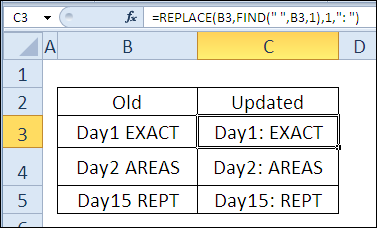
For day 27 in the challenge, we’ll examine the SUBSTITUTE function. Like the REPLACE function, it replaces old text with new text, in a text string, but can replace multiple instances of the same text.

In some situations though, it’s quicker and easier to use the Find/Replace command on the Excel Ribbon, with Match Case option turned on, for case sensitive replacement.

So, let’s take a look at the SUBSTITUTE information and examples, and if you have other tips or examples, please share them in the comments.

Function 27: SUBSTITUTE

The SUBSTITUTE function replaces old text with new text, in a text string. It will replace all instances of the old text, unless a specific occurrence is selected, and SUBSTITUTE is case sensitive.

How Could You Use SUBSTITUTE?

The SUBSTITUTE function replaces old text with new text, in a text string, so you could use it to:

• Change region name in report title
• Remove non-printing characters
• Replace last space character

SUBSTITUTE Syntax

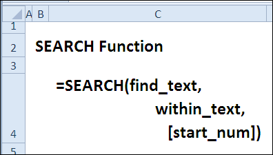
The SUBSTITUTE function has the following syntax:

• SUBSTITUTE(text,old_text,new_text,instance_num)
  • text is the text string or cell reference, where text will be replaced.
  • old_text is the text that will be removed
  • new_text is the text that will be added
  • instance_number is the specific occurrence of old text that you want replaced

SUBSTITUTE Traps

• The SUBSTITUTE function can replace all instances of the old text, so use the instance_num argument if you want only a specific occurrence of old text replaced.
• For replacements that are not case sensitive, you can use the REPLACE function.

Example 1: Change region name in report title

With the SUBSTITUTE function, you can create a report title that changes automatically, based on the region name that is selected.

In this example, the report title is entered in cell C11, which is named RptTitle. The “yyy” in the title text will be replaced with the region name, selected in cell D13.

=SUBSTITUTE(RptTitle,”yyy”,D13)

Example 2: Remove non-printing characters

When you copy data from a website, there might be hidden, non-printing space characters in the text.

If you try to remove space characters from the text in Excel, the TRIM function can’t remove them. The characters aren’t normal space characters (character 32); they are non-breaking space characters (character 160).

Instead, you can use the SUBSTITUTE function to replace each of the non-printing spaces with a normal space character. Then, use TRIM to remove all the extra spaces.

=TRIM(SUBSTITUTE(B3,CHAR(160),” “))

Example 3: Replace last space character

Instead of replacing all instances of a text string, you can use the SUBSTITUTE function’s instance_number argument to select a specific instance. In this list of recipe ingredients, we want to replace the last space character only.

In cell C3, the LEN function calculates the number of characters in cell B3. The SUBSTITUTE function replaces all the space characters with empty strings, and the second LEN function finds the length of the revised string. The length is 2 characters shorter, so there are two spaces.

=LEN(B3)-LEN(SUBSTITUTE(B3,” “,””))

In cell D3, the SUBSTITUTE function replaces only the 2nd space character with the new text – ” | ”

=SUBSTITUTE(B3,” “,” | “,C3)

Instead of using two columns for this formula, you could combine them into one long formula.

=SUBSTITUTE(B3,” “,” | “,LEN(B3)-LEN(SUBSTITUTE(B3,” “,””)))

Download the SUBSTITUTE Function File

To see the formulas used in today’s examples, you can download the SUBSTITUTE function sample workbook. The file is zipped, and is in Excel 2007 file format.

Watch the SUBSTITUTE Video

To see a demonstration of the examples in the SUBSTITUTE function sample workbook, you can watch this short Excel video tutorial.

_____________

Yesterday, in the 30XL30D challenge, we changed text strings with the REPLACE function, and learned that it can insert characters too.

OFFSET function

For day 26 in the challenge, we’ll examine the OFFSET function. From a starting reference, it returns another reference, of a specified size, and offset by a set number of rows and columns.

So, let’s take a look at the OFFSET information and examples, and if you have other tips or examples, please share them in the comments.

Function 26: OFFSET

The OFFSET function returns a reference offset from a given reference.

How Could You Use OFFSET?

The OFFSET function can return a reference to a range, and be combined with other functions. Use it to:

• Find sales amount for selected month
• Sum the selected month’s sales
• Create a dynamic range based on count
• Sum the last n month’s sales

OFFSET Syntax

The OFFSET function has the following syntax:

• OFFSET(reference,rows,cols,height,width)
  • reference is a cell or range of adjacent cells.
  • rows can be positive (below starting reference) or negative (above starting reference)
  • cols can be positive (right of starting reference) or negative (left of starting reference)
  • height must be positive, and is number of rows in returned reference
  • width must be positive, and is number of columns in returned reference
  • if height or width are omitted, starting reference size is used

OFFSET Traps

The OFFSET function is volatile, so it could slow down a workbook if used in too many cells. Instead, you could use another function, like INDEX, to return a reference.

Example 1: Find sales amount for selected month

With the OFFSET function, you can return a reference to a range, based on a starting reference. In this example, we want the sales amount in cell G2:

• starting reference is cell C1
• number of rows to offset is entered in cell F2
• sales amount is in column C, so the number of columns to offset is zero
• height is 1 row
• width is 1 column

=OFFSET(C1,F2,0,1,1)

In cell H2, there is a similar OFFSET formula, to return the month name. The only difference is the column offset — 1 instead of zero.

=OFFSET(C1,F2,1,1,1)

Note: The height and width arguments could be omitted, because we want a reference that is the same size as the starting reference. I used them in this example, to show how all the arguments work.

Example 2: Sum the selected month’s sales

In this example, the OFFSET function returns a reference to the sales amounts for the selected month, and the SUM function returns the total for that range.

In cell B10, the selected month number is 3, so the result is the total of the March sales.

• starting reference is A3:A6
• rows to offset is zero (you could omit the zero, for the same result)
• columns to offset is entered in cell B10
• height and width are omitted, because the reference should be the same size as the starting reference

=SUM(OFFSET(A3:A6,0,B10))

Example 3: Create a dynamic range based on count

You can also use the OFFSET function to create a dynamic range. In this example, I’ve created a name, MonthsList, with this formula:

=OFFSET(‘Ex03’!$C$1,0,0,COUNTA(‘Ex03’!$C:$C),1)

If another month is added to the list in column C, it will automatically appear in the data validation drop down list in cell F2, which uses MonthsList as its source.

Example 4: Sum the last n month’s sales

In this final example, OFFSET is combined with SUM and COUNT, to show the total for the last n months. As new quantities are added, the formula result will automatically adjust to include the latest months.

In cell E2, the number of months is 2, so the August and September amounts are summed.

• starting reference is cell C2
• number of rows to offset is calculated by counting numbers in column C, subtracting number in cell E3, adding 1
• quantity is in column C, so the number of columns to offset is zero
• height is entered in cell E3
• width is 1 column

=SUM(OFFSET(C2,COUNT(C:C)-E3+1,0,E3,1))

Download the OFFSET Function File

To see the formulas used in today’s examples, you can download the OFFSET function sample workbook. The file is zipped, and is in Excel 2007 file format.

Watch the OFFSET Video

To see a demonstration of the examples in the OFFSET function sample workbook, you can watch this short Excel video tutorial.

_____________

Yesterday, in the 30XL30D challenge, we got cell addresses with the ADDRESS function, and combined it with INDIRECT to get a cell’s value.

TYPE Function

For day 21 in the challenge, we’ll examine the TYPE function. It identifies the type of value in a cell, by returning a number.

So, let’s take a look at the TYPE information and examples, and if you have other tips or examples, please share them in the comments.

Function 21: TYPE

The TYPE function returns a number, that identifies a value’s type:

Here’s the list of results, and the data types:

How Could You Use TYPE?

The TYPE function can tell you what kind of value is in a cell, but the logical functions, like ISERROR, ISTEXT, etc., will also check for a specific data type.

However, if you just want to know what’s in a cell, the TYPE function can:

• Identify cell value type by number
• Test for Number type before multiplying

TYPE Syntax

The TYPE function has the following syntax:

• TYPE(value)
  • value can be text, number, error, or any other value

TYPE Traps

Unfortunately, the TYPE function cannot identify cells that contain a formula. It only shows the type for a cell’s contents, or a formula’s result.

In a few versions of Excel, the Help files incorrectly reported that a formula would return 8 with the TYPE function. This MSKB article corrects that error.

https://support.microsoft.com/kb/119148

Example 1: Identify cell value type by number

The TYPE function returns number, based on a value’s type, so you can use it to see what’s in a cell. For example, if you type 123 in cell B3, the result of this formula is 1 — Number.

=TYPE(B3)

However, if there is an apostrophe in front of the number, the TYPE function result would be 2 — Text.

Example 2: Test for Number type before multiplying

You could use the TYPE function with CHOOSE, to multiply valid numbers, or show a message, if something else is entered.

=CHOOSE(MIN(TYPE(B3),3),B3*C3,”No text”,”Enter Qty”)

• If a number is entered in B3, the TYPE function returns 1, so the CHOOSE function returns the result of B3*C3.

• If text is entered in B3, the TYPE function returns 2, so the CHOOSE function returns the message “No text”.

• If anything else is entered in B3, the TYPE function returns a 4 or higher. The MIN function result will be 3, so the CHOOSE function returns the message “Enter Qty”.

Download the TYPE Function File

To see the formulas used in today’s examples, you can download the TYPE function sample workbook. The file is zipped, and is in Excel 2007 file format.

Watch the TYPE Video

To see a demonstration of the examples in the TYPE function sample workbook, you can watch this short Excel video tutorial.

_____________

Yesterday, in the 30XL30D challenge, we found text strings with the SEARCH function, and used IFERROR and ISNUMBER to deal with its error results.

MATCH Function

For day 19 in the challenge, we’ll examine the MATCH function. It searches for a value in an array, and returns its position, if the value is found.

To see a the MATCH function sample workbook, you can watch this short video. There are written steps below the video

Function 19: MATCH

The MATCH function returns the position of a value in an array, or #N/A if not found. The array can be sorted, or unsorted, and the MATCH function is not case sensitive.

How Could You Use MATCH?

The MATCH function returns the position of an item in an array, and that result can be used by other functions, such as INDEX or VLOOKUP. For example:

• Find position of item in unsorted list
• Use with CHOOSE to get student grades
• Use with VLOOKUP for flexible column choice
• Use with INDEX for to show winner’s name

MATCH Syntax

The MATCH function has the following syntax:

• MATCH(lookup_value,lookup_array,[match_type])
  • lookup_value can be text, number or logical value
  • lookup_array is an array, or array reference (contiguous cells in a single row or column)
  • match_type can be -1, 0 or 1. If omitted, assumed to be 1

MATCH Traps

MATCH function returns the position of the item found, not the value. If you need the value, combine MATCH with another function, like INDEX.

Example 1: Find Item in Unsorted List

For an unsorted list, you can use 0 as the match_type argument, to find an exact match. If you’re searching for text, and using 0, you can include wildcard characters in the lookup value.

In this example, you can type a month name, or partial name with wildcards, to find that month’s position in the list.

=MATCH(D2,B3:B7,0)

Instead of an array reference, you can enter an array as the lookup_array argument.

In this variation, the lookup month name is entered in cell D5, and three month names are entered in the MATCH function’s second argument.

If a later month, such as Oct, is entered in D5, the result will be #N/A.

=IF(C2+0<14,”Time to upgrade”,”Latest version”)

Example 2: Change Student Grades to Letters

Just as you did with VLOOKUP, you can use MATCH to help convert a student’s score to a letter grade. In this example, it is combined with CHOOSE, to get the letter grade. The match_type is -1, because the scores are sorted in descending order.

When the match_type is -1, the result is the smallest value greater than or equal to lookup value. The lookup value is 54, and it’s not in the list of scores, so the position for 60 is returned.

Because 60 is in position 4, the 4th value in the CHOOSE options is the result — cell C6, with a value of D.

=CHOOSE(MATCH(B9,B3:B7,-1),C3,C4,C5,C6,C7)

Example 3: Create Flexible Column Choice in VLOOKUP

To make a VLOOKUP formula more flexible, you can use MATCH to find a column number, instead of hard-coding it into the formula.

In this example, users can select a region in cell H1, as the value for the VLOOKUP. Then, they can select a Month in cell H2, and the MATCH function returns the column for that month.

=VLOOKUP(H1,$B$2:$E$5,MATCH(H2,B1:E1,0),FALSE)

Example 4: FIND Closest Match with INDEX

The MATCH function also works well with the INDEX function, which we’ll see later in the challenge.

In this example, the MATCH function is used to find the guess that is closest to the correct number.

1. The ABS function returns the absolute difference between each guess and the correct number.
2. The MIN function finds the smallest difference.
3. The MATCH function finds the smallest difference in the list of differences. If there are multiple identical differences, the first one will be returned.
4. The INDEX function returns the name in that position in the list of names.

=INDEX(B2:B5,MATCH(MIN(ABS(C2:C5-F1)),ABS(C2:C5-F1),0))

Download the MATCH Function File

To see the formulas used in today’s examples, you can download the MATCH function sample workbook. The file is zipped, and is in Excel 2007 file format.

Watch the MATCH Video

To see a demonstration of the examples in the MATCH function sample workbook, you can watch this short Excel video tutorial.

_____________