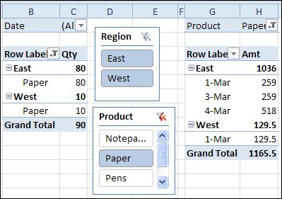
In Excel 2007, and earlier versions, you can use Excel VBA code if you want to automatically filter multiple pivot tables at the same time. That task is much easier in Excel 2010, thanks to the new Slicer feature.
ISREF and the IS Functions — although it sounds like the name of a geeky band, it’s not. Today we’ll take a look at ISREF, which is one of the 9 IS functions that are lumped together in the Excel Help files.
How sad — 9 functions that never get to shine on their own. We’ll give ISREF a few minutes in the spotlight, to see how it works.
The Excel IS Functions
The following IS functions are listed on one page in Excel Help:
ISBLANK(value)
ISERR(value)
ISERROR(value)
ISLOGICAL(value)
ISNA(value)
ISNONTEXT(value)
ISNUMBER(value)
ISREF(value)
ISTEXT(value)
They all work in the same way — the function tests a value, and returns TRUE if the value passes the test.
NOTE: There is also a new ISFORMULA function for Excel 2013 and later versions.
IS Function Examples
For example, if cell B2 contains a number, the ISNUMBER formula will result in TRUE:
=ISNUMBER(B2)
ISNONTEXT Function Excample
If cell B3 contains anything except text, even if cell B3 is blank, the ISNONTEXT formula will result in TRUE:
=ISNONTEXT(B3)
ISNONTEXT Function Example
The other IS functions work the same way, and give the expected results — except for ISREF.
ISREF Function Problems
In the screen shot below, there is a reference in cell B2, with the following formula: =D1
In cell D2, the ISREF function returns TRUE as the result.
However, the ISREF function also returns TRUE in cell D3, even though there is a typed value in cell B3 — the number 7
How ISREF Function Works
The ISREF function isn’t testing what’s in the referenced cell, it’s testing the reference within the formula.
And because the ISREF formulas in both D2 and D3 contain references, the result is TRUE for both formulas.
So, the ISREF function won’t help you assess whether there is a reference another cell.
ISREF Uses
If you can’t use ISREF to detect a reference in another cell, how can you use it?
Well, ISREF can check the results of other formulas, to see if they have returned a valid reference.
You could use ISREF, instead of ISERROR, in your formulas that need references.
For example, in the screen shot below, the INDIRECT function in cell D2 returns a reference, and INDIRECT(“D1”) creates a valid reference.
If cell B2 contains the text “D1”, this formula results in TRUE:
=ISREF(INDIRECT(B2))
ISREF With OFFSET
The first OFFSET formula in the screen shot below is not valid, because there is no cell that is 1 column to the left of cell A1, so the ISREF result is FALSE
=ISREF(OFFSET(A1,0,-1))
Hoever, the second OFFSET formulas returns a valid reference to cell B1, so the ISREF result is TRUE.
Any Other Uses for ISREF Function?
Do you use ISREF in your formulas? Can you think of any other examples for using it?
______________ Save
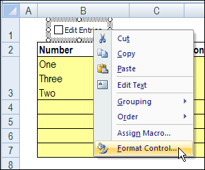
A couple of years ago, I described how you could select multiple items from an Excel drop down list. One of my clients needed that feature in a workbook last week, so I’ve made an enhancement to the VBA code. Now you can edit multiple selections in Excel after entering them.
Last Friday, there was an HLOOKUP example, and it used a dynamic lookup range — as rates were added to the lookup table, it automatically expanded to include them.
You probably use defined names in some of your Excel workbooks. We’ll look at a built-in way to list the names in a workbook, and see some Excel VBA code that creates a more detailed list of names.
For example, if you have entered a list of the products that you sell, you could select the list, and name the range reference as ProdList.
Then, that product list could be used in an order form.
Table Names
If you created Excel Tables, in Excel 2007 or Excel 2010, they are automatically named.
Later, you can change the names to something meaningful, such as ProdTable, for a list of products and their prices.
Create a List of Names
If you’re working on a complex Excel workbook, it’s easy to lose track of what you’ve named, and where the named ranges are located.
For reference, you can print out a list of names, using a built-in feature in Excel.
To paste a list of workbook level names in Excel:
Insert a blank worksheet
On the Excel Ribbon, click the Formulas tab
In the Defined Names group, click Use in Formula, and click Paste Names (the keyboard shortcut is F3)
paste a list of workbook level names in Excel
Paste Name Dialog Box
Next, in the Paste Name window, click the Paste List button.
Paste Name Dialog Box
Names List on Worksheet
A list of defined names and their formulas is pasted into the worksheet.
Note: To see worksheet level names, use the Paste List feature on the worksheet where those names are defined.
Create Names List with Excel VBA Macro
The built-in names list feature is helpful, but if you need more details, you can create your own list, by using Excel VBA.
This macro adds a new sheet to the active workbook, with a list of the non-hidden defined names, with details for each name, if available.
A – Name;
B – Refers To formula;
C – Number of cells in the range;
D – Sheet name where range is located;
E – Address on worksheet;
F – Scope (workbook or worksheet)
Sub ListAllNames()
Dim lRow As Long
Dim nm As Name
Dim wb As Workbook
Dim ws As Worksheet
Dim wsL As Worksheet
Dim wsName As String
Dim shName As String
Dim myName As String
Dim nmRef As String
Dim nmAddr As String
Dim nmRng As Range
Dim nmSc As String
Dim lCells As Long
Set wb = ActiveWorkbook
Set ws = ActiveSheet
Set wsL = Worksheets.Add

wsName = ws.Name

With wsL
    .Range("A1:F1").Value = Array("Name", _
        "Refers To", "Cells", "Sheet", "Address", "Scope")
    lRow = 2
End With

On Error Resume Next
  For Each nm In wb.Names
    If nm.Visible Then
      Set nmRng = nm.RefersToRange
      myName = nm.Name
      nmRef = "'" & nm.RefersTo
      lCells = nmRng.Cells.Count
      shName = nm.RefersToRange.Parent.Name
      nmAddr = nm.RefersToRange.Address
      If TypeOf nm.Parent Is Workbook Then
        nmSc = "Wb"
      Else
        nmSc = "Ws"
      End If
      wsL.Range(wsL.Cells(lRow, 1), wsL.Cells(lRow, 6)).Value _
         = Array(myName, nmRef, lCells, shName, nmAddr, nmSc)
      lRow = lRow + 1
      Set nmRng = Nothing
      myName = ""
      nmRef = ""
      lCells = 0
      shName = ""
      nmAddr = ""
      nmSc = ""
    End If
  Next nm

With wsL
  .Rows("1:1").Font.Bold = True
  .Columns("A:F").EntireColumn.AutoFit
End With

End Sub
Download the Names List Sample File
To get the sample workbook, and the Names List code, go to the Excel Names Macros page on my Contextures site.
The file is zipped, and in Excel xlsm file format, and it contains macros.
___________
There is an Excel weekly meal planner on the Contextures website, in which you can select meal items, and create a weekly shopping list.
Excel Weekly Meal Planner Shopping List
Shopping List Problems
In December, I added an online recipe selector, created by Jimmy Peña, and described the new feature in a blog post.
This weekend, Alyssa pointed out a problem — if you select a meal item twice, it’s only added to the shopping list once.
That could cause problems, if you run out of food on Friday, and have hungry and cranky children waiting for their dinner. Thanks Alyssa!
Fix the List
To show the correct quantities in the shopping list, I changed the heading in the original quantity column, from Qty to Meal Qty.
Then, I added a new column, with the heading Qty, and a formula to multiply the Meal Qty by the List qty.
The formula in cell H2 multiplies the Meal Qty by the List Qty:
=C2*G2
That should prevent any food shortages at the end of the week!
Download the Updated Excel Meal Planner
You can see the full details for the Excel Weekly Meal Planner on the Contextures website, and download an updated copy to help plan your meals.
____________
On Day 10 of the 30 Excel Functions in 30 Days series, we looked at the Excel HLOOKUP function. It’s similar to VLOOKUP, but looks for values in a horizontal list, instead of a vertical list.
The second example in that HLOOKUP blog post showed how to find a rate in a lookup table, based on the date entered in cell C5. On March 15th, the rate would be 0.25, because the Jan 1st rate is still in effect.
Beyond One Cell
In the comments for the HLOOKUP blog post, Fred said that he got the formula working correctly in cell D5, but wondered how to use the result in multiple cells.
In this example, we’ll use the rates as a lookup for pricing. The prices change quarterly, and the correct price will be used in each order, based on the order date.
Set Up the Lookup Table
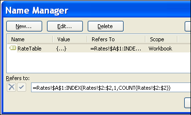
In this workbook, the table with the quarterly dates and rates is on a separate sheet, named Rates.
New rates will be added each quarter, so we’ll create a dynamic range named RateTable, using the technique from Example 3 in the 30XL30D INDEX function post.
In this HLOOKUP rates table, the formula for the named range is:
In the Orders table, we’ll use an Excel HLOOKUP formula to pull the correct rate from the RateTable range, based on the order date.
In cell B2, the formula is:
=HLOOKUP(A2,RateTable,2)
The final argument is omitted, so the result is an approximate match.
If the order date isn’t found in the first row of the RateTable range, the HLOOKUP formula result is based on the next largest date that is less than order date.
Add the Pricing Formula
The final step is to add the pricing formula in column D. Quantities will be entered in column C, so the pricing formula will multiply the quantity by the rate.
The formula in cell D2 is:
=B2*C2
Download the Sample File
To see the Excel HLOOKUP formula and the RateTable named range, you can download the HLOOKUP Rates sample file.
It is in Excel xlsx format, and zipped.
_______________
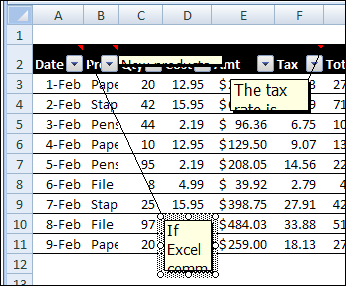
Do you ever open an Excel workbook, and find that tragedy has struck your comments? You spent hours inserting those comments, and making them just the right size and shape. Then, for no apparent reason, everything changes. Comments are in the wrong place, and wrong size. Here’s how to fix those wandering Excel comments.
Yes, it’s Valentine’s Day today, and if you were too busy to buy your sweetie a card yesterday, you can make one in Excel. Phew!
Your boss won’t mind if you spend a couple of hours working on this today, because it’s an Excel project! This Excel Valentine card uses a named range, data validation, a formula, and conditional formatting (to change the heart from white to pink to red).
If you won’t have time, or if your drawing skills are worse than mine, you can download the sample Excel Valentine file, at the end of this blog post.
And if you want some romantic music in the background, while you work on your Excel Valentine card, you can listen to the YouTube playlist, compiled by John Walkenbach and his blog readers.
Set Up the Worksheet
To create the heart shape,
Start by making columns A:M narrower, to create square cells
Then, add red fill colour to cells in rows 5:14, to create a heart shape
Tip: To type a heart shape, press Alt and type a 3 on the number keypad (if no number keypad, try Fn+Alt+L). On a Mac, another key combination might be needed.
Use the Excel Valentine
The Excel Valentine heart has white fill and white font, so it’s not visible.
To see the heart:
Select one item from the drop down lists, to colour the valentine light pink
Select two items from the drop down lists, to colour the valentine dark pink
Select three items from the drop down lists, to colour the valentine red


 There is an

 On Day 10 of the 30 Excel Functions in 30 Days series, we looked at the Excel


 Yes, it’s Valentine’s Day today, and if you were too busy to buy your sweetie a card yesterday, you can make one in Excel. Phew!


