Excel Price Lookup: VLOOKUP or INDEX

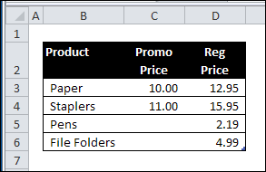
This week, Glen emailed me for advice on extracting prices from a lookup table. Some products have a promotional price each month, but other products are sold at the regular price.

Pricing Lookup Table

I’m blocking email attachments these days, so I can’t show you the exact setup of Glen’s Excel worksheet.

However, a simplified version might look something like this:

Pricing Lookup Table

Use VLOOKUP to Find Pricing

In his email, Glen mentioned that he is using a VLOOKUP formula.

  • If there is a promotional price, he wants VLOOKUP to return the value from the Promo Price column.
  • If there is no promotional price, Glen wants the price from the Regular Price column.

Use IF Function

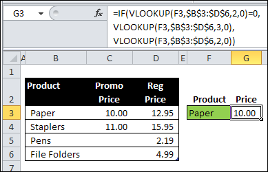
To do that, Glen could use the IF function, with VLOOKUP:

=IF(VLOOKUP(F3,$B$3:$D$6,2,0)=0,
VLOOKUP(F3,$B$3:$D$6,3,0),
VLOOKUP(F3,$B$3:$D$6,2,0))

IF function with VLOOKUP

CHOOSE the Right Price

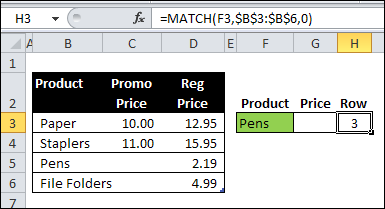
Another option is to use the MATCH function to find the row that the product is in.

In the screen shot below, the following formula is in cell H3:

=MATCH(F3,$B$3:$B$6,0)

use the MATCH function to find the row

CHOOSE and INDEX Functions

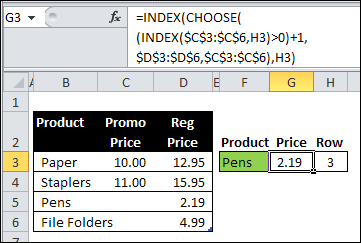
Next, in cell G3, use the CHOOSE function and the INDEX function, to get the correct price:

=INDEX(CHOOSE((INDEX($C$3:$C$6,H3)>0)+1,
$D$3:$D$6,$C$3:$C$6),H3)

PromoPrice04

How the CHOOSE Formula Works

In this example, the CHOOSE function selects the correct pricing column to use for the prices. The outer INDEX function returns the price from the selected column.

First, the inner INDEX function returns the price from the promo column, for the selected product, and we check to see if the price is greater than zero:

INDEX($C$3:$C$6,H3)>0

  • If there is NO promo price, the result is FALSE (0)
  • If there IS a promo price, the result is TRUE (1)

Next, we add 1 to that result, so

  • FALSE=1
  • TRUE=2.

CHOOSE the Range

Next, the CHOOSE function returns a reference to the selected range.

  • FALSE (1) = $D$3:$D$6
  • TRUE (2) = $C$3:$C$6

Finally, the first INDEX function returns a price from the selected column, in the row for the selected product.

How Would You Solve the Problem?

I’m sure there are several other ways to solve Glen’s lookup problem. What formula would you use?
________________

Desert Island Excel Files

image Over the past few days, I’ve been without my desktop computer, which is on its way back to the repair shop.
Fortunately, most of my files were available on the external hard drive, and online storage, so there were no major catastrophes. Well, none that I’ve discovered yet!

Personal Macro File

Unfortunately, my personal Excel macros add-in file wasn’t backed up, so I had to work without it for a while.

You don’t realize how often you use something, until it’s missing!

Your Desert Island Excel Files

My Excel tip for you today is – Remember to back up ALL your Excel files, including the add-ins, toolbars, and other key files.

Imagine that you and your laptop will be abandoned on a desert island.

  • Do you have everything installed that you’ll need for Excel survival?
  • Or will you be voted off the island?

Check Your Backup System

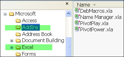
Make sure your backup system is copying files from the C:Documents and Settings/YourName/Application Data/Microsoft folder, such as the Addins and Excel files.

Check Your Backup System

Island Internet Access

And let’s hope that desert island has internet access, so you can send email to your clients, and use the files that you have stored in your online storage folders!

What are your desert island backup plans?
__________

See the Secret Excel Error Number

I’ve been working with Excel for approximately 125 years, and never realized that there was a hidden number in the worksheet error messages.

Excel Error Message

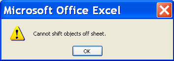
For example, if you try to insert a column in Excel, you might see this message that warns “Cannot shift objects off sheet“.

shiftobjectserror01

See Error Message Number

To see the specific error number for that message, you can press the following keyboard shortcut:

  • Ctrl + Shift + I

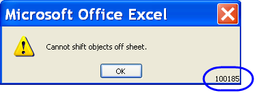
The error message number appears in the bottom right corner of the error message. I’ve circled the number in the screen shot below.

Error Message Number shows after shortcut used

Use the Error Number

That error message number could be useful if you’re doing a Google search, to find a solution to a specific problem.

Or, that number could be useful if you’re searching in the Microsoft Knowledgebase, or anywhere on the Microsoft website, for specific help.

Did you know those error numbers were hidden in the messages?
_________________

Excel Function Friday: Subtotal and Sumproduct with Filter

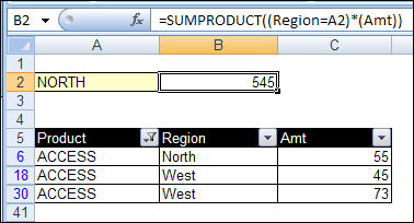
Last week, we used the Excel SUBTOTAL function to sum items in a filtered list, while ignoring the hidden rows. Now we’ll look at ways to use Subtotal and SumProduct with filter settings applied.

Continue reading “Excel Function Friday: Subtotal and Sumproduct with Filter”

Excel Function Friday: Sum Filtered List With SUBTOTAL

The Excel SUM function does a great job of adding numbers on a worksheet, and it’s probably the first Excel function that you learned about.

But SUM might not be the best function to use in all situations where you need a total.

Continue reading “Excel Function Friday: Sum Filtered List With SUBTOTAL”