Filter Pivot Charts in Excel 2010

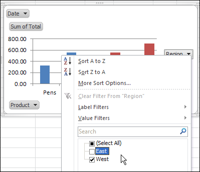
In Excel 2007, there was a PivotChart Filter Pane, and you had to open that if you wanted to filter the pivot chart. Things have improved in Excel 2010, and the PivotChart Filter Pane is gone.

Excel Pivot Charts

After you create a pivot table in Excel, you can insert a pivot chart, based on that pivot table.

• Note: If you need help with creating a pivot chart, there are step-by-step instructions on the Pivot Chart Source Data page of my Contextures site.

Pivot Chart Field Names

The field names now appear on the pivot chart, which is great news! Each field button has a drop down arrow, and you can use those drop downs to quickly and easily add or clear the filters.

Types of Pivot Chart Field Buttons

There are four different types of field buttons for pivot charts:

1. Report Filter Field Buttons
2. Legend Field Buttons (pivot table Column fields)
3. Axis Field Buttons (pivot table Row fields)
4. Value Field Buttons

Show or Hide Buttons

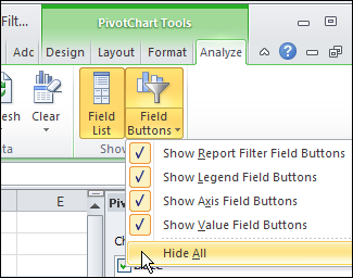
You can show or hide the individual field buttons, or use the Hide All command on the Ribbon, to control what appears in the pivot chart.

Watch the Pivot Chart Filter Video

To see the steps for creating and filtering a pivot chart in Excel 2010, you can watch this short Excel tutorial video.

The full transcript is below the video.

Video Transcript: Use Field Buttons to Filter Pivot Chart

Pivot charts have improved in Excel 2010 and I’m going to show you the new filtering feature which is much easier than it was in Excel 2007.

Insert Pivot Chart

To insert a pivot chart, I’m selecting a cell in the pivot table.

And then, on the Ribbon, under Pivot Table Tools, I’ll click Options.

And in the Tools group, click PivotChart

I’m going to select a Column chart type

And the first one here, which is the Clustered Column

And click OK

That inserts a chart right on the active worksheet.

I can point to one of the corners of the chart and make it a bit smaller

Filter Pivot Chart

And to filter now, I can use any of the field buttons, that are on the chart.

So if I only want to see a specific product or date, then I can click the arrow and filter right in the pivot chart.

So perhaps I just want to see April 7th

And that filters both the chart and the pivot table.

Remove Pivot Chart Filters

To remove the filters, I can go back, and click All

And that shows all the data again.

Show or Hide Field Buttons

There’s also a setting on the Ribbon, if you go to PivotChart Tools, and click Analyze.

There is a Field Buttons setting, that you can show or hide specific buttons, that are on the chart, or hide all of them.

More Pivot Chart Info

Excel Pivot Charts

Pivot Chart Source Data

Pivot Table Slicers

________________