
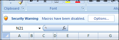
Occasionally, I get calls from clients who don’t understand why their Excel file isn’t working. They’re clicking buttons, or selecting from drop down lists, but none of the usual magic is happening. Is the file broken?
Unmerge Excel Cells
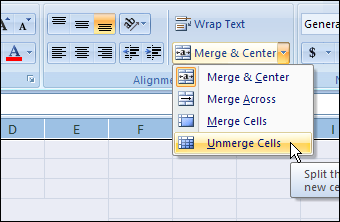
I saw this on Twitter yesterday: Wanted “Break Apart all merged cells in entire spreadsheet” button. If you’ve done much work in Excel, you’ve probably encountered problems that are the result of merged cells on a worksheet.
Merging cells can seem like a good idea at the time, but can interfere with sorting and filtering, and other things that make an Excel workbook useful. Here’s how you can unmerge Excel cells.
Temporarily Hide Excel Conditional Formatting
To highlight specific cells on an Excel worksheet, you can use conditional formatting.
In the example shown below, orders with a quantity greater than 50 are highlighted with green fill colour.

Conditional Formatting Rule
This was the result of simple conditional formatting, based on the cell value.
Sometimes though, the conditional formatting can be distracting, and there’s no built in way to temporarily remove it.

Create an On/Off Switch
Instead of removing the conditional formatting, you could add an On/Off switch to your worksheet. Then, adjust the rules, so you only show the conditional formatting when the switch is on.
In the screenshot below, there’s a cell named CondF_Show, and it has a data validation drop down for Yes and No.

Change Conditional Formatting Rule
I changed the conditional formatting to a formula that checks both the Quantity cell value, and the value in the CondF_Show cell.

On/Off Switch Set to No
After you revise the rule, when the CondF_Show cell is changed to No, the conditional formatting is temporarily hidden.

More Conditional Formatting Info
For more Conditional Formatting rules and advanced examples that use a formula, go to the Conditional Formatting Examples page on my Contextures site.
And here are a few more pages on my site, where you can learn more about Excel Conditional Formatting:
Fix Conditional Formatting Extra Rules
Conditional Formatting – Currency
Conditional Formatting – Documentation
Conditional Formatting – Data Bars
____________
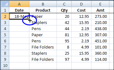
Excel VLOOKUP in Different Ranges
You can use the VLOOKUP function to find data in a lookup table, based on a specific value. If you enter a product number in an order form, you can use a VLOOKUP formula to find the matching product name or price. See how to use Excel VLOOKUP in different ranges.
NOTE: The examples below use VLOOKUP to get the value from the correct table. You could do a similar lookup with the INDEX and MATCH functions.
AutoFill Excel Dates in Series or Same Date
If you’re entering dates on an Excel worksheet, you don’t have to enter each date individually. Just enter the first date, in the top cell. Then, if there is data in the next column, you can use the Fill handle to quickly enter the rest of the dates. See how to AutoFill Excel dates in series or same date, with just a couple of clicks.
Continue reading “AutoFill Excel Dates in Series or Same Date”
Drag a Text File Into Excel
Last month, I showed you how to drag information from a web browser into Excel.
Here’s the very short video that I posted, in case you missed it.
Drag Text Files Into Excel
You can also drag text files, to open them quickly in Excel.
I find this a really quick way to open a text file, especially if Windows Explorer is already open.
Drag Text File From Windows Explorer
Instead of using the Open command, or the Text Import Wizard, just drag a text file into the Excel window.
In the screen shot below, Windows Explorer is already open.
I’m dragging the text file, named MyDataFix.txt, onto the active Excel worksheet

Text File Data on Worksheet
After I drop the text file onto the worksheet, the text file opens automatically.
In the screen shot below, the data appears in separate columns in the worksheet, because the data was saved in a tab separated format.

___________
Pivot Table Formatting Old Style
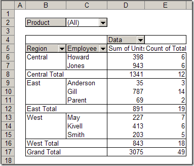
Today, we’ll look at pivot table formatting, old style, but first, here’s an update. In the last blog post, you saw how to turn off buttons and drop downs in an Excel 2007 pivot table, and there are a couple of updates on that topic.
Hide Pivot Table Buttons and Labels
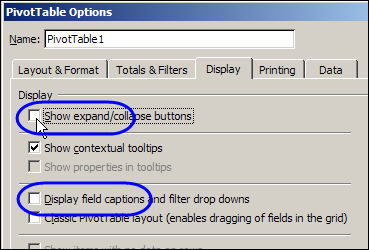
If you’re sharing an Excel pivot table with colleagues who aren’t too skilled in Excel, you might want to hide some of the pivot table buttons and labels before you send it.
Continue reading “Hide Pivot Table Buttons and Labels”
Trouble Aligning Excel Currency Symbols
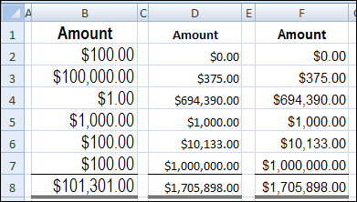
Every now and then I get a workbook from a client with numbers in Accounting format. If all the numbers are the same length, the currency symbols line up nicely. However, if the numbers are different lengths, we have trouble aligning Excel currency symbols.
Shorten Data Validation List With Excel Filter Macro
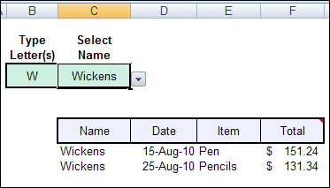
An Excel data validation drop down list only shows 8 items at a time, and with a long list of items, it might take you a while to scroll through that long list.
To make data entry easier, see how to shorten data validation list, by using a macro.
Continue reading “Shorten Data Validation List With Excel Filter Macro”