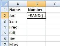
Here’s how I ran a small contest, and what I did to pick a winner from a list of names in Excel.
Continue reading “Pick a Winner From a List of Names in Excel”
Excel tips and tutorials

Here’s how I ran a small contest, and what I did to pick a winner from a list of names in Excel.
Continue reading “Pick a Winner From a List of Names in Excel”
Do people email you, asking for Excel help? Co-workers? Family members? Strangers from the Internet?
Here’s a favourite “Email Help” message from my mailbox this week:
Subject: help me in excel
Dear sir,
I have a problem in excel i requesting to you solve this. I am sending the data of excel sheet pls look in to that
If you have want any information on that please get back to me
I am waiting for your reply
Regards
Anonymous
Those “Dear Sir” emails make me feel like Peppermint Patty. At least the attached Excel file was small, unlike some of the multi-megabyte files I’ve been sent.
Sorry Anonymous, but I can’t help with your Excel problem today. My desk is piled high with work, and I won’t have any extra time to decipher your file.
Fortunately, there are places where Anonymous, or you, can get free help with your Excel problems, or ask questions about other Microsoft products.
These are much better options than emailing me, and asking for private help. Why?
Good luck, Anonymous! I hope you find someone who can help with that Excel question.
_______________________
“Help!” said the familiar voice, when I picked up the phone at 10 PM.
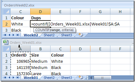
“I have a list of orders in an Excel sheet. I want to compare it with the list from last week, and delete all the orders that were in the old list.”
It was my daughter, still at the office, trying to get a pile of work done before the looming deadline. I helped her with a COUNTIF formula, and she was able to leave for home a short time later. Phew!
The first step is to check each OrderID in the new list, to see if it’s also in the old list.
We’ll use a COUNTIF formula to calculate how many times each OrderID is found in the old list. If the count is zero, we know it’s a new order.


We can see that the first three numbers in the new list are also in the old list, and they have been correctly counted as 1.
The next three numbers aren’t in the old list, so their count is zero.

Now that the new orders are identified with a zero, we can delete the old orders.


See how to use Excel COUNTIF function to count cells in a list that contain specific words or part of a word. For example, how many orders were for a Pen? How many orders for any kind of pen, such as “Gel Pen”, “Pen” or even a “Pencil”?
There are more Excel counting tips on the Contextures website.
For more examples of using the Excel COUNTIF function, see these blog posts:
Check Winning Numbers with COUNTIF
Use COUNTIFS for Multiple Criteria
Quickly Change COUNTIF Criteria
Count Cells Greater Than Set Amount
____________________________
Have you ever had trouble trying to count items in an Excel list, based on two criteria? See how to use the Excel SUMPRODUCT function to get the count that you need
Instead of using the COUNT function, or the COUNTA funtion, you can use the SUMPRODUCT function to count items based on 2 criteria.
In the example shown below, the SUMPRODUCT function is used to count the rows where :
This solution will work in any version of Excel, including Excel 2003 or earlier, where there COUNTIFS function is not available.

Instead of typing the criteria in a formula, you can refer to a cell, as shown in the second formula below.
=SUMPRODUCT(–(A2:A10=”Pen”),–(B2:B10>=10))
2. Or use cell references:
=SUMPRODUCT(–(A2:A10=D2),–(B2:B10>=E2))
There are many more examples, written steps, and videos for counting in Excel on my Contextures website.
Count Criteria in Other Column
Count Cells With Specific Text
____________
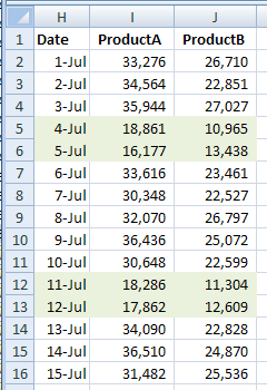
Yes, the weekend is over, but another one is just five days away! To make it easier to keep track of Saturdays and Sundays, you can use conditional formatting to highlight weekend dates in Excel.
In an exclusive World Movie Premiere, here is the first (and probably last) instalment in Excel Theatre. It’s an animated short, named Absolute Reference Problems. Watch for it in this year’s Oscar nominations!
Please note the giant spreadsheet in the background of the video below. I think that grid adds to the tension in this dramatic presentation.
Just so you know – the video’s dialog is corny, the actors are wooden, the plot is weak and the costumes are pitiful. Other than that, it’s pretty good. 😉
If you haven’t used INDIRECT before, it’s a formula that returns a reference to a range, based on a text string.
As the video pointed out, you can use an absolute reference to a cell, to “lock” the reference, and keep if from changing if you copy the formula to a different cell.
However, if the referenced cell moves, the absolute reference changes to match the new location.
For example, in the screenshot below:

If you insert a blank row at the top of the worksheet, the formula in cell C2 changes, and it now refers to cell A2.
However, because it’s a text string, the reference in the INDIRECT formula does NOT change. It returns a zero because cell A1 is now empty.

You can use INDIRECT in many ways. For example:
For more information on the INDIRECT function, and examples of how to use it, please visit the INDIRECT Function page on my website.
In case you want to read along with the animated video characters, here is the full transcript. Have fun!
Oh No!
What is wrong?
I used an absolute reference to cell A1
Good! Your formula should always refer to that cell
I thought so too, but then I inserted a new row at the top of the worksheet
That should be okay
It isn’t! Now my formula refers to cell A2
Oh no! The total could be wrong now.
How could that happen? What is the point of using an absolute reference if it can change?
Maybe you should try an INDIRECT instead
D’oh! Why didn’t I think of that?
I will change it to an INDIRECT formula, and it will always refer to cell A1, thanks!
How did I end up making this silly Excel video? Well, I should have been working all day, but decided to take a bit of time to relax and catch up on some reading (of RSS feeds).
On a technology blog, I saw a link to XtraNormal, where you can write, cast and direct an animated movie.
That sounded like more fun than working, so off I went.
________________
In a pivot table, you might want to see all the orders that were shipped on a specific date.
To do that, you’d move the Ship Date field to the Page area, and select a date from the drop down list.

Sometimes though, you’d like to show the orders shipped in a date range, instead of just a single date. For example, you might like to show orders with ship dates in the upcoming week, so you can do some planning.
To accomplish this, you could manually hide all the dates in the Ship Date page field, except the dates for next week. However, that might take quite a while if there are lots of dates.
Another option is to add a new field to the source data, to test the ship dates, then add it to the pivot table, as a filter. This might slow things down a bit, if your source data table is very large.
We’ll look at both options in Excel 2003 — the steps are slightly different in Excel 2007.
In Excel 2003, there are no check boxes beside the items in a Page field’s drop down list, to allow you to select multiple items.
To hide some of the items in a pivot table’s Page field, temporarily move the field to the Row area, and select the items there, then drag the date field back to the Page area.

Or, without moving the field in the Page area, you can change the field’s settings.

Manually hiding the dates might work well if you only need to do this occasionally, and the list of dates isn’t too long. Otherwise, the best solution might be to add a column to the pivot table’s source data.
In this case, we’ll add a column named ShipSoon, and use a formula to test if the ship date is within the next 10 days.
=AND(A2>TODAY(),A2<=TODAY()+10)

Each row will show TRUE or FALSE as the result of the formula.
Next, you’ll update the pivot table, and add the new field.

Remember to refresh the pivot table each day to see the current calculations for the ShipSoon field.

Or, you can set the pivot table to automatically refresh when you open the Excel file.

____________________
Do you have two or more web pages that you use frequently? I like Google as a home page, and use it many times during the day.
I also refer to my own website several times, to make sure everything is working okay, or look up one of the Excel tips that are stored there.
I had Google set as my home page in Firefox, then opened Contextures.com later.

It’s not a terribly painful process, but I’ve found a way to set multiple home pages, instead of one.
Here’s how I set up the multiple pages:

The next time you open Firefox, both home pages will automatically open.
_______________________
Usually when I use VLOOKUP, I want to pull information for an exact match.
For example, if I enter a customer number in one cell, I want the customer name in the adjacent cell. I don’t want the name of a customer whose number is CLOSE to the one that I entered.
Continue reading “Excel VLOOKUP-Change Percent to Letter Grade”
Today’s challenge was to create a table of contents in Excel, for a downloaded price list.
The data came from Crystal Reports and had formatting on the section headings.
Some of the headings were repeated, but we didn’t want the TOC to include the duplicates.

I’ve created a table of contents based on sheet names, in other workbooks, but hadn’t tried to index a sheet’s contents.
In this case, all the heading cells were blue, so I decided to write a macro that would create a TOC entry for any blue cell.
A quick test in the Immediate window showed me the colour index — 42.

The macro that I wrote does the following steps:
The price list has a few hundred product categories, so that Autofilter makes it easier to find the product that you want.

Here’s the Excel VBA code that I wrote, and you can add your own error handling.
You can also download the sample Hyperlink TOC file (Excel 2007 format).
Sub CreateHyperlinks()
Dim c As Range
Dim ws As Worksheet
Dim wsTOC As Worksheet
Dim lRowTOC As Long
Dim lColor As Long
Dim strTOC As String
Dim strHead As String
lRowTOC = 2
lColor = 42
strTOC = "TOC"
strHead = ""
On Error Resume Next
Application.DisplayAlerts = False
Worksheets(strTOC).Delete
Application.DisplayAlerts = True
On Error GoTo 0
Set wsTOC = Worksheets.Add
With wsTOC
  .Name = strTOC
  .Cells(1, 1).Value = "Product"
  .Cells(1, 1).Font.Bold = True
End With
For Each ws In ThisWorkbook.Worksheets
  If ws.Name <> strTOC Then
    For Each c In ws.UsedRange.Columns(1).Cells
      If c.Interior.ColorIndex = lColor Then
        'don't index duplicate headings
        If strHead <> c.Value Then
          wsTOC.Cells(lRowTOC, 1).Value = c.Value
          wsTOC.Hyperlinks.Add _
          Anchor:=wsTOC.Cells(lRowTOC, 1), _
          Address:="", _
          SubAddress:=c.Parent.Name _
          & "!" & c.Address, _
          TextToDisplay:=c.Value
          lRowTOC = lRowTOC + 1
          strHead = c.Value
        End If
      End If
    Next c
  End If
Next ws
wsTOC.Columns(1).AutoFilter
wsTOC.Columns(1).AutoFit
End Sub
___________________