Happy Thursday! I’ve got two news items today, and you can read the details below.
- a new sample file on my Contextures website
- a Microsoft Consumer Camp event in the Toronto area
Continue reading “Change Pivot Table Filters With Drop Down Cell”
Excel tips and tutorials

Happy Thursday! I’ve got two news items today, and you can read the details below.
Continue reading “Change Pivot Table Filters With Drop Down Cell”
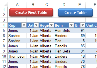
A few years ago, Excel MVP Kirill Lapin shared his code to create a pivot table from identically structured tables in two or more Excel files. His technique used a Union query in Microsoft Query, and you can see the details here.
Continue reading “Create Pivot Table or Excel Table from Multiple Files”
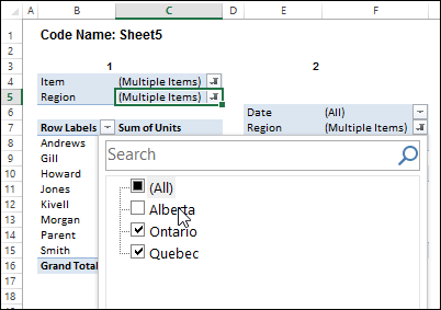
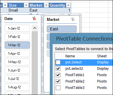
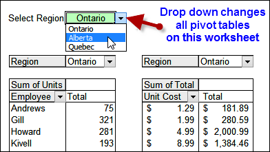
In the screen shot below, one of the report filters in a pivot table is about to be changed. If you have multiple pivot tables in a workbook, you can use programming to update all (or some) of the pivot tables, if one pivot table’s filters are changed.
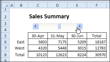
A couple of months ago, I shared an example with a scroll bar that selects the dates for an Excel report. There is a pivot table on a hidden sheet, and a summary report uses GetPivotData formulas to pull data from that pivot table.
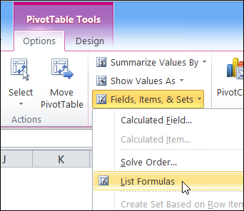
A few months ago, I shared my code for listing all the formulas in an Excel workbook. The code creates a new worksheet, with details on each formula’s worksheet name, cell address, the formula and the formula in R1C1 format.
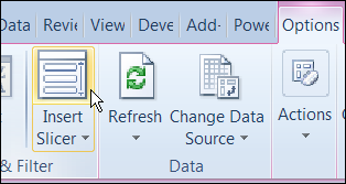
Slicers were introduced in Excel 2010, and they make it easy to change multiple pivot tables with a single click.
Note: In earlier versions, you can use programming to change the report filters in multiples pivot tables.
Recently, I enrolled in an online Infographics and data visualization course, and the classes started last week. In one of my homework assignments, I used this trick to link pivot chart title to report filter.
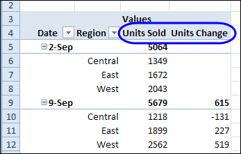
A pivot table is a great way to summarize data, and most of the time you probably use a Sum or Count function for the values. For example, in the pivot table shown below, the regional sales are totaled for each week. We can also use a built-in feature to calculate differences in a pivot table.
In Excel 2010, you can use Slicers to change multiple pivot tables. However, you might be working in an earlier version of Excel, or you don’t have room for Slicers on your worksheets.
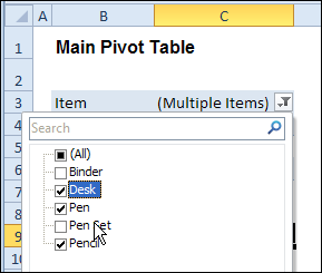
Instead of Slicers, you can use programming to update multiple pivot tables automatically. In previous posts, I’ve shown how you can select items in one pivot table’s Report Filter fields, and the Report Filter fields for pivot tables on the other worksheets will change to the same selections.
Jeff Weir has written an updated version of the code, which runs much faster than the previous version. You’ll notice the speed difference especially if you’re working with larger pivot tables.
Also, in this version of the code, you can specify:
For example, only update the pivot tables on Sheet1 and Sheet2, and ignore PivotTable2 on Sheet1.
[Update: Sept 20, 2012] Jeff has made the following changes to the code:
Jeff is also working on a version of the code for Excel 2010, that promises to be even faster — so stay tuned for that!
[Update: June 16, 2013] Jeff has revised the code, so it uses Slicers if the version is Excel 2010 or later.
In the previous version of the code, it looped through each master pivot field multiple times, to determine if each pivot item is visible or hidden. The corresponding pivot item in each secondary pivot table was then set to the same setting. The code worked, but it was very slow in larger pivot tables.
The main reason that Jeff’s code is faster is that it iterates through each master pivot field just once, so it can record only the visible items into a dictionary.
Then, for each pivot field in each secondary pivot table:
Also, speed in Jeff’s code is increased because it:
If you download the sample file (see instructions below), you can copy the code to your own workbooks.
Here is where you’ll change the sheet names in the SyncPivotFields code:

Here is the section where you’ll change the pivot table names:

To download this version of the sample file, with Jeff’s code, please visit the Sample Files page on the Contextures website.
Note: Jeff’s sample file was updated on Sept. 20, 2012, so please download the new version if you have an older copy of the file.
In the Pivot Tables section, look for: PT0029 – Change Pivot Table Fields on Specific Sheets
The file is in Excel xlsm format, zipped, and contains macros. Enable the macros when opening the file, if you want to test the code.
__________________
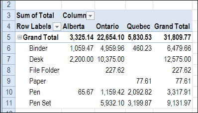
In a pivot table, you can choose to show or hide the grand totals, but you can’t change their position. However, with a quick and easy workaround (no programming required), you can show the grand total at top of pivot table, for rhe pivot table columns.