Category: Pivot Table

An Excel pivot table is a great way to summarize a large amount of data, and with its Top 10 filter, you can compare the top values to the bottom values.

But don’t limit yourself to the Top 10 versus the Bottom 10 – dig deeper by using the other options in the filter.

Summarize the Data

With a few mouse clicks, you can summarize thousands of rows of data into a concise and informative pivot table.

In this example, there is a list of product, and their total sales over two years.

Sort by Sales Values

Instead of viewing the products alphabetically, you can sort by total sales, in descending order, to see the best selling products at the top of the list.

Here is the same list, with Oatmeal Raisin at the top.

Spotlight the Best Selling Products

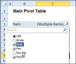
Instead of showing all the products, you can use the pivot table’s Top 10 filter in the Product field, to filter the results.

The Top 10 filter is customizable, and can be used to show the top 3 items, instead of the top 10.

Top 3 Sales in Pivot Table

Here is the pivot table, with the Top 3 items showing, and the grand total for those items.

Compare to Bottom Items

If you’re working on a sales plan, you might want to decide where to focus your efforts, and a pivot table, or two, could help.

• If the top 3 products have total sales of approximately $136K, how are the bottom selling products doing, in comparison?
• How many of those bottom selling products are required to match the top 3 sales?

To find out, you can make a copy of the pivot table, and change the Top 10 filter. Instead of Top 3 Items, filter for Bottom Sum, and use the $136K amount as the target SUM.

Difference in Comparison Results

In this example, the top 3 sales were $136,165, and the bottom 10 products have sales of $173,489. The totals are not an exact match, because the pivot table filters for the products that total the specified sum, or more.

Find Best Results

The bottom 9 products don’t reach the target amount, so the 10th lowest product is also included. That puts the total over the target, and it shows that the best results come from a small number of products.

Focus your sales efforts there, and you might have a great sales year.

Watch the Pivot Table Top 10 Compare Video

To see the steps for comparing top and bottom values in a pivot table, you can watch this short Excel video tutorial.

________________

To format a pivot table, you can select a specific section, such as one of the fields, or a grand total. When you point to a field heading, a black arrow will appear, if the Enable Selection setting is turned on.

Black Arrow Pointer

In the screen shot below, you can see the black arrow at the top of the Product field. Click in that spot, and all the Product item labels are selected.

Click in that spot again, and the Product heading is selected, instead of the item labels.

Pivot Table Field Setting Quick Tip

Instead of a single click on a heading cell, you can point to an outer field heading and double-click when the black arrow appears.

In the screen shot below, the black arrow is on the Bran product heading cell.

Note: This trick won’t work on an inner field, like Region, which has no other fields under it.

Open Field Settings

Double-click on the outer field heading, and the Field Settings dialog box opens.

In there, you can change the layout and other settings, and add or remove subtotals.

Right-Click Menu

Another way to open the Field Settings dialog box is to right-click on an item, and click Field Settings in the popup menu. This works for both inner and outer fields in the pivot table.

I find the double-click shortcut to be quicker and easier – as long as you remember to point somewhere that the black arrow appears.

Watch the Pivot Table Selection Video

To see the steps for selecting section of an Excel Pivot Table, you can watch this short video tutorial.

_________________

In Excel 2010, you can use Slicers to change the filters in several pivot tables, with a single click.

If you don’t have Excel 2010, or don’t want to use Slicers, you can use programming to change multiple pivot table filters with a single click.

Yes, it’s more work than adding a Slicer, but better than manually changing all those pivot tables!

Change All Pivot Tables

Last December, I described how to add code to your workbook, so if you changed one pivot table filter, all the other pivot tables in the workbook would change too.

Click here to read that article, and the comments: Change All Pivot Tables With One Selection

In those comments, people asked how to modify the code, so only the pivot tables on the active sheet were affected, or only a specific field was changed.

In response to those comments, I’ve created a new version of the sample file.

Change All Pivot Tables or Active Sheet Only

The latest sample file for changing pivot table fields has 3 variations on the “Change All Page Fields” code.

It also changes the “Multiple Item Selection” settings to match changed page fields (Excel 2007 and Excel 2010 only).

The three variations are:

1. Change any page field in a pivot table, and all matching page fields, on all sheets, are changed.
2. Change any page field in a pivot table, and all matching page fields, on the active sheet only, are changed.
3. Change a specific page field in a pivot table, and that page field, on the active sheet only, is changed.

Download the Sample File

To see the code, and try the variations, you can download the sample file from the Contextures website. The file will work in Excel 2007 or Excel 2010, if you enable macros.

PT0027 – Change All Page Fields – All Sheets or Active Sheet

You can also download the other sample files, showing how to change a specific field, or all fields, in the workbook’s pivot tables.

PT0008 – Change Multiple Page Fields

PT0015 – Change Multiple Different Page Fields

PT0016 – Change Page Fields With Cell Dropdown

PT0021 – Change All Page Fields

PT0025 – Change All Page Fields with Multiple Selection Settings

______________

Yesterday, i created a custom PivotTable Style for a customer, to make it easy to format multiple pivot tables, using their corporate colour scheme.

PivotTable Styles are available in Excel 2010 and Excel 2007, and if you don’t like the existing styles, you can create your own custom styles, and apply those to any pivot table.

Copy Custom PivotTable Styles

Unfortunately, there’s no built in way to copy a custom PivotTable style from one workbook to another.

A while ago, I made this video, to show you a workaround for copying your favourite styles to a different workbook.

Remove Existing Formatting

If you’re applying a built-in or a custom style to a pivot table, you might need to remove any manually applied formatting first.

• Instead of clicking on the PivotTable Style icon, right-click on it.
• Then, click Apply and Clear Formatting

You might need to tidy up the pivot table after you apply the new style, but with Custom Styles you can quickly format your pivot tables, so they have a consistent appearance.

______________________

If you have similar data on two or more worksheets, you might want to combine that data in a pivot table, to show the summarized results.

Unfortunately, the pivot table from data on multiple sheets can be a disappointment.

Create a Pivot Table with Programming

A couple of years ago, Excel MVP, Kirill Lapin (KL), shared a sample file that he created, with amendments by Hector Miguel Orozco Diaz.

It uses code to automatically create a pivot table from multiple sheets in a workbook.

You can read the details here: Create a Pivot Table from Multiple Sheets.

Revised Solution

Kirill’s sample file was created as a conceptual prototype, and targeted advanced VBA users. The code has minimal error handling and compatibility checks.

However, the sample file was extremely popular, and Excel users at all skill levels wanted to adopt this solution in their own applications. To make things easier, Kirill has created a similar solution based on ADO.

Advantages:

1. No need for temporary file generation
2. The code is faster and less prone to errors

Disadvantages:

1. No manual refresh of the PivotTable
2. Need to rebuild connection from the scratch to update the cache with new data

Download the ADO Sample File

You can download the new ADO version of the file from the Contextures website: PT0024 – Pivot Table from Multiple Sheets – ADO version.

There is also a “Plug and Play” version of the file, at the same link.
________________

This week, I was updating the GetPivotData Function page on my website, and remembered how hard it was to turn off that feature, in Excel 2003 and earlier.

We won’t even talk about the really olden days (Excel 2000), when you had to type those tricky GetPivotData formulas yourself!

Automatic Formulas

If you try to reference a pivot table cell, a GetPivotData formula may be automatically created, instead of a simple cell reference. This is thanks to the Generate GetPivotData feature, which is turned on by default.

The automatic formula can be a helpful feature, but sometimes you’d rather just have the cell link. You could type the link yourself, or find a way to turn off the formula feature.

GetPivotData in Excel 2003 and Earlier

In the old versions of Excel, if you want to stop that automatic formula creation, you have to add the Generate GetPivotData button to the PivotTable toolbar.

If you’re nostalgic for the old method, you can see it in the video at the end of this blog.

GetPivotData in Excel 2007 and Excel 2010

Now, it’s much easier to turn the Generate GetPivotData feature on and off.

1. Select any cell in a pivot table.
2. On the Excel Ribbon, under PivotTable Tools, click the Options tab.
3. In the PivotTable group, click the drop down arrow for Options
4. Click the Generate GetPivotData command, to turn the feature on or off.

GetPivotData Formulas

There is more information on the GetPivotData Function page, including examples of using cell references within the formula.

It’s a great way to pull specific data from your pivot tables.

Generate GetPivotData Button in Excel 2003

To see how we changed this setting in the olden days, you can watch this short video.

___________