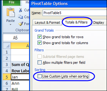
Usually, it’s easy to sort an Excel pivot table – just click the drop down arrow in a pivot table heading, and select one of the sort options. Occasionally though, you might run into pivot table sorting problems, where some items aren’t in A-Z order.
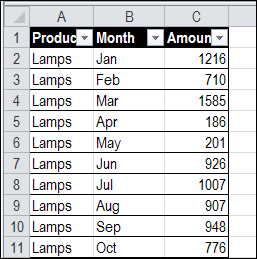
If your Excel data is in monthly columns, like the worksheet shown below, you’ll have trouble setting up a flexible pivot table. Instead of leaving the data like this, see how to normalize data for Excel pivot table setup.
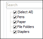
One way to let users change the function is to create a drop down list of functions on the worksheet. Then, event code runs when the cell changes, and the selected function is shown in the pivot table.
The cell with the drop down list is named FuncSel, as you can see in the NameBox in the screen shot above.
On another sheet, that could be hidden from the users, there is a list of functions, and a formula that looks up the numeric value for each function. The cell with the formula is named FuncSelCode.
How It Works
When the FuncSel cell is changed, the Worksheet_Change code on that sheet runs.
Private Sub Worksheet_Change(ByVal Target As Range)
If Target.Address = Me.Range("FuncSel").Address Then
    ChangeAllData (wksLists.Range("FuncSelCode").Value)
End If
End Sub
The ChangeAllData procedure runs, using the numeric value in the FuncSelCode cell, and changes all the data fields in the pivot table.
Sub ChangeAllData(lFn As Long)
'changes data fields to selected function
On Error GoTo errHandler
Dim pt As PivotTable
Dim pf As PivotField
Dim ws As Worksheet
Application.ScreenUpdating = False
Set pt = wksPTSales.PivotTables(1)
On Error GoTo errHandler
pt.ManualUpdate = True
For Each pf In pt.DataFields
  pf.Function = lFn
Next pf
pt.ManualUpdate = False
exitHandler:
Set pf = Nothing
Set pt = Nothing
Application.ScreenUpdating = True
Exit Sub
errHandler:
GoTo exitHandler
End Sub
With the pivot table Show Details feature in Excel, a new sheet is inserted when you double-click on the value cell in a pivot table.
It’s a great feature for drilling into the details, but you can end up with lots of extra sheets in your workbook.
Usually, you don’t want to save the sheets, so you manually delete them before you close the file.
Automatically Name the Sheets
With event code on the pivot table’s worksheet, and in the workbook module, you can add a prefix – XShow_ – when these detail sheets are created.
That prefix should make the sheets easier to find and delete.
Automatically Delete the Sheets
To make the cleanup task even easier, you can use event code to prompt you to delete those sheet when you’re closing the workbook.
If you click Yes, all the sheets with the XShow_ prefix are deleted. Then, click Save, to save the tidied up version of the workbook.
See the Drilldown Sheet Code
For detailed instructions on adding the drilldown sheet naming and deleting code, visit the Excel Pivot Table Drilldown page on the Contextures website.
Download the Sample Drilldown File
To see how the event code names the sheets, and deletes them when closing, you can download the Pivot Table Drilldown sample file.
________________
In the comments of the previous article, James asked how to keep those Slicers from overlapping the pivot tables.
Does anyone know how to stop slicers moving around when you make selections. This happens if the slicers are viewed on top of the pivot table data. As the pivot output data shrinks or expands the slicers move around and sometimes obscure each other. Any idea how to fix in place?
Pivot Table Update Event
One way to fix the problem of sliding Slicers is to automatically move the Slicers, any time the pivot table is updated.
To do that, you can use the PivotTableUpdate event, and a macro that moves the Slicer to the right side of the pivot table.
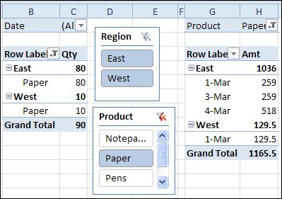
Slicer Caption
Each Slicer has a caption, and you can refer the the Slicer by that caption in the Excel VBA code.
In this example, the Slicer has a caption of “Region”, which is shown at the top of the Slicer.
The caption is also visible on the Excel Ribbon’s Options tab, when the Slicer is selected.
Slicer caption visible on Excel Ribbon’s Options tab
Macro to Move a Pivot Table Slicer
Here is the sample code that I used.
This macro moves a pivot table slicer to the right side of the pivot table, any time the pivot table is updated.
Sub MoveSlicer()
    Dim wsPT As Worksheet
    Dim pt As PivotTable
    Dim sh As Shape
    Dim rngSh As Range
    Dim lColPT As Long
    Dim lCol As Long
    Dim lPad As Long
    Set wsPT = Worksheets("PivotSales")
    Set pt = wsPT.PivotTables("PivotDate")
    Set sh = wsPT.Shapes("Region")
    lPad = 10
    lColPT = pt.TableRange2.Columns.Count
    lCol = pt.TableRange2.Columns(lColPT).Column
    Set rngSh = wsPT.Cells(1, lCol + 1)
    sh.Left = rngSh.Left + lPad
End Sub
How the Code Works
In the code, a variable (pt) is set for the pivot table.
The code counts the columns in the pivot table’s TableRange2 range, which includes the Report Filters area. (TableRange1 does not include the report filters.)
lColPT = pt.TableRange2.Columns.Count
The code adds 1 to the column number that the last pivot table column is in.
Set rngSh = wsPT.Cells(1, lCol + 1)
A variable (lPad) sets the padding number — how much the Slicer will be moved to the right. In this example, the variable is set to 10
lPad = 10
Finally, the Slicer is positioned, in the column to the right of the pivot table. In that column, the Slicer’s left side is indented by the padding amount.
sh.Left = rngSh.Left + lPad
Pivot Table Update Code
The following code should be copied to the pivot table’s worksheet module.
It will run the macro to move a pivot table slicer (MoveSlicer), any time the PivotDate pivot table is updated.
Private Sub Worksheet_PivotTableUpdate(ByVal Target As PivotTable)
    If Target.Name = "PivotDate" Then
        MoveSlicer
    End If
End Sub
Download the Sample File
To see how the macro to move a pivot table slicer works, you can download the Excel Slicer Move Code sample workbook. The file is in xlsm format, and is zipped. You’ll have to enable macros, to test the code.
_______
There is a page on the Contextures website that describes how to clear old items in pivot table drop downs. Someone ran into a problem with that code, and here’s how we fixed it.
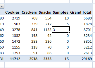
One of my clients uses a pivot table to summarize product sales, using sales data from their accounting system. Occasionally, they’d like to type a number in the pivot table, but Excel won’t let you change values in a pivot table. Here is a workaround for that limitation.
In Excel 2007, and earlier versions, you can use Excel VBA code if you want to automatically filter multiple pivot tables at the same time. That task is much easier in Excel 2010, thanks to the new Slicer feature.


 Recently, we saw how you can