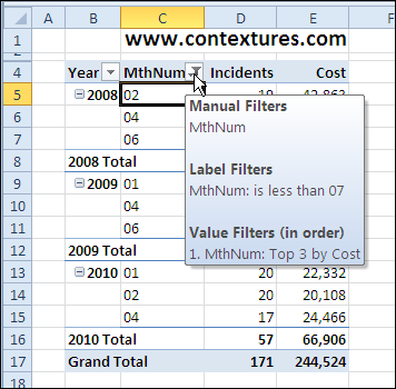
One of the best features of a pivot table is filtering, which allows you to see specific results in your data. See which types of filters are available, and learn how you can apply more than one filter on pivot table field at the same time.
If you’re looking for love, move along — the “Canadian Singles” in the article title refers to hit songs, not eligible bachelors.
Last week, a new book was published with a list of top 100 Canadian singles, based on a poll of music professionals and fans.
In his J-Walk blog, John Walkenbach posted a link to the Canada’s Top 100 Singles list, and there was a lively discussion in the comments section.
Top 100 Canadian Singles List
No discussion is complete without a spreadsheet, so I copied the list into Excel, and cleaned it up.
To make it more interesting, I found the release date for each hit song, and split them into decades, using the Excel FLOOR function.
Make a Pivot Table
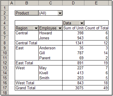
From that data, I created a pivot table, showing the count of songs from each decade, listed by rank.
Was most of the best music released in the 1970s, or were most of the voters from that era?
Pivot Table Song Count by Decade
Pivot Table Group Numbers by 10
In column A, the top 100 songs are grouped by 10s, to summarize the data.
For example, row 5 shows the decade counts for the songs ranked from one to ten in the top 100 list.
Group numbers by 10 in pivot table
Highlight with Color Scale
Next, I added conditional formatting to highlight the decades with the largest number of songs.
Repeat Pivot Table Item Labels
A new feature in Excel 2010 pivot tables is the ability to repeat the field item labels.
In another copy of the pivot table, I put the decade in the row label area, and changed the pivot table report layout to Outline Form.
Change Pivot Field Setting
Then, I right-clicked on the Decade field, and clicked Field Settings. On the Layout & Print tab, I added a check mark to Repeat Item Labels, and clicked OK.
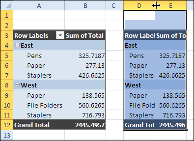
After changing that setting, the decade is repeated in each row, instead of showing just once, at the top of the section.
Repeat Pivot Table Item Labels
Download the Top 100 Canadian Single File
To see the list, and create your own pivot table, you can download one of my sample files.
To keep your data details confidential, you might want to send someone a copy of a pivot table, without the link back to its source data. It’s easy to copy a pivot table, and paste it as values,but it is difficult to copy pivot table format and values.
You can use the PowerPivot add-in for Excel 2010 to create a report from multiple Excel workbooks or worksheets, by joining the tables using the Primary and the Foreign key, such as ‘ProductID’ in a Sales table and a Pricing table.
I promised you a second pivot table macro, and here it is. In today’s example, Kirill combines data from a sales list and price list, stored in separate workbooks.
The macro combines the data and calculates the selling price for each item, then creates a pivot table from the results.
If you want to create a pivot table from data on different worksheets, you can use a Multiple Consolidation Ranges pivot table. However, that creates a pivot table with limited features and functionality.
My friend and client, Bob Ryan, from Simply Learning Excel, has just published a hands-on, no fluff, Excel book — Simply Learning Excel 2007: Learn the Essentials in 8 Hours or Less.
To celebrate the book launch, I asked Bob to share one of his favourite Excel tips with you, and you can read Bob’s answer below.
Bob’s Pivot Table Macro
Bob Ryan’s top Excel tip:
Some time ago, I was getting ready to train a group of people about PivotTables. As I was documenting the steps, I started feeling more and more annoyed at the number of steps it took to create the kind of PivotTable I typically use.
So, I wrote a macro to automate the steps. (I also submitted a suggestion to Microsoft to allow users to create a customized standard/default PivotTable, but I don’t see it in Excel 2010.)
I wanted to share this macro, but since my website is generally geared to folks who don’t know about or need macros (yet), I asked Debra if I could be a guest writer, and she kindly agreed.
A final note: While I appreciate Debra’s willingness to share this information on her site, the content really belongs to her because most of this information came from her books, website, and/or her personally. I hope you find this useful.
What the Macro Does
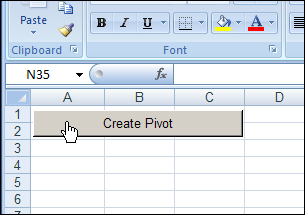
Once you insert a PivotTable and enter a field(s) into the Values area, the code does the following to PivotTable(1) on the active sheet:
Applies the Classic PivotTable display, with gridlines and no colors (I like this so I can Copy the PivotTable and Paste Special Values and Formatting.);
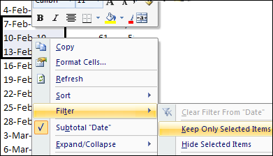
Ensures that only data that still exists in the data that drives the PivotTable will appear in the PivotTable dropdown lists.
Sets all fields to ascending order with no subtotals, including fields that are not in the Row Labels or Column Labels areas, and;
For the data field(s) in the Values area, changes the setting to Sum, changes the number format, and, if the field in the Values area is named “Amount” or “Total Amount” it shortens the label in the PivotTable to “Sum Amt” or “Sum TtlAmt” respectively.
The file is zipped, and in Excel 2007 format. Because it contains a macro, you’ll have to enable macros when you open the file.
Watch the Video
Thanks, Bob, for sharing your pivot table macro!
To see how much time you can save by using a macro to format a pivot table, watch this video.
It took me a couple of minutes to manually format the Excel pivot table, and change some of the pivot table options, and just a couple of seconds to do all the same steps with Bob’s macro.
Note: If you record your own pivot table formatting macro, follow Bob’s example to add variables, so the macro works on any pivot table, no matter what the field names are, or where it’s located.
About the Author
Robert Ryan, MBA, CPA is a long-time passionate user of Excel, the author of “Simply Learning Excel 2007: Learn the Essentials in 8 Hours or Less,” a unique step-by step book designed for basic to intermediate users, and the host of “Ask the Author… LIVE!™” where Bob answers questions from readers of his book in live WebEx sessions at no extra cost.
How can you get missing data to show up in your Excel pivot table, showing a count of zero? AlexJ encountered this problem recently, and sent me his solution, to share with you.
If you’re working with an Excel pivot table, you might want to temporarily hide one or more of the items in a Row field or Column field. To do that, you probably click the drop down arrow for the Row or Column Labels, then remove the check mark for items you want to remove.
Today, we’ll look at pivot table formatting, old style, but first, here’s an update. In the last blog post, you saw how to turn off buttons and drop downs in an Excel 2007 pivot table, and there are a couple of updates on that topic.

 If you’re looking for love, move along — the “Canadian Singles” in the article title refers to hit songs, not eligible bachelors.