Many moons ago, Dave Peterson created a sample Excel worksheet data entry form and kindly shared it on the Contextures website.
In Dave’s original form, users could add records on the data entry sheet, and click a button to go to the database sheet, where they could review or edit the order records.
If you’re on the second sheet, you can click the Next button to go to the third sheet.
Or, click the Back button to go to the first sheet.
Excel worksheet navigation buttons
Check for Hidden Sheets
In the comments for that blog post, Ron de Bruin suggested modifying the two navigation macros, so they test if the target sheet is hidden, before selecting it.
Finally, only 14 months later, the revised code is ready. As you know, quality work takes time! 😉
Excel Worksheet Navigation Code
Here’s the Excel VBA code for the two macros — GoSheetBack and GoSheetNext.
If the next sheet is hidden, the code keeps going until it finds the next visible sheet.
If the macro code reaches the end of the sheet tabs in either direction, it jumps to the other end, and continues from there.
'==========================
Sub GoSheetNext()
Dim wb As Workbook
Dim lSheets As Long
Dim lSheet As Long
Dim lMove As Long
Dim lNext As Long
Set wb = ActiveWorkbook
lSheets = wb.Sheets.Count
lSheet = ActiveSheet.Index
lMove = 1
With wb
  For lMove = 1 To lSheets - 1
    lNext = lSheet + lMove
    If lNext > lSheets Then
      lMove = 0
      lNext = 1
      lSheet = 1
    End If
    If .Sheets(lNext).Visible = True Then
      .Sheets(lNext).Select
      Exit For
    End If
  Next lMove
End With
End Sub
'==========================
Sub GoSheetBack()
Dim wb As Workbook
Dim lSheets As Long
Dim lSheet As Long
Dim lMove As Long
Dim lNext As Long
Set wb = ActiveWorkbook
lSheets = wb.Sheets.Count
lSheet = ActiveSheet.Index
lMove = 1
With wb
  For lMove = 1 To lSheets - 1
    lNext = lSheet - lMove
    If lNext < 1 Then
      lMove = 0
      lNext = lSheets
      lSheet = lSheets
    End If
    If .Sheets(lNext).Visible = True Then
      .Sheets(lNext).Select
      Exit For
    End If
  Next lMove
End With
End Sub
'==========================
Download the Sample File
To see the detailed instructions, and to download the sample Navigation code workbook, please go to the Excel VBA Worksheet Macro Buttons page on the Contextures website.
Watch the Excel Video
To see the steps for creating the navigation macro buttons, you can watch this Excel video.
Last week, someone wrote and asked how to modify that code, so only a specific user could add new items. Everyone else should see a message that says they aren’t permitted to add items.
This technique isn’t foolproof, and anyone who’s determined to circumvent it would be able to. But, it’s a good way to remind people that they can’t update the list without permission.
Identify the User
One way to find out who’s trying to add a new item, is to check the user name that’s entered in the Microsoft Office application.
After you install Office, you can personalize it in Excel Options, in the Popular category, by entering your name in the User Name box.
User Name box in Excel Options
In Excel VBA, you can create variables to capture that user name, and the name of the authorized user:
    Dim strAuth As String
    Dim strUser As String
    strAuth = "Debra Dalgleish"
    strUser = Application.UserName
Block Non-Authorized Users
After you figure out who the user is, you can block them from doing something. In this workbook, we want to block all but one user from adding new items.
    If strUser <> strAuth Then
        MsgBox "You do not have authority to add Work Order numbers. " _
            & vbCrLf _
            & vbCrLf _
            & "Please check with Administrator before continuing."
        GoTo exitHandler
Remove the Added Item
The above code will block people from adding the new item to the data validation drop down, but doesn’t prevent them from typing the new item in the data validation cell. With another line of code, you can undo the invalid entry that they made.
        Application.Undo
        GoTo exitHandler
Disable Events
Because the code might make a change on the worksheet, you’ll have to turn off the EnableEvents property. That will prevent the Worksheet_Change code from running again, while it’s in the middle of running the first time.
At the top of the procedure, add the line to turn off the EnableEvents property.
Application.EnableEvents = False
In the exitHandler, remember to turn EnableEvents back on.
If you’ve added comments to an Excel worksheet, you have a couple of built-in options for printing the comments.
Show the comments on the worksheet, and print them as displayed.
Print the list of comments at the end of the worksheet, on a separate printed page.
Printing Comments Shown on Sheet
Printing the comments on the worksheet is okay if there are only a couple of comments, and you can arrange them so they don’t cover the data.
comments shown on the worksheet
Print List of Comments
For more than a couple of comments, the list at the end of the worksheet is a better choice.
However, with the built-in list printing option, you just get the cell address and comment, printed in a long, single column.
Create Your Own List of Comments
Instead of using the built-in list of printed comments, you can use a macro to create your own list of comments on a separate worksheet, and print that list.
It’s also a great way to review all the comments on a worksheet, and use sorting or filtering to focus on specific comments.
Create Your Own List of Comments
See the Comment Printing VBA Code
Shown below is the Excel VBA code to create a list of comments from the active sheet, written by Dave Peterson.
For more comment programming examples, including Dave’s code to list all the comments in the entire workbook, see Excel Comments VBA.
The Comment List Code
The ShowComments macro adds a new sheet to the workbook, and lists all the comments, the comment author name, and the comment cell’s value, address and name (if any).
At the end of the macro, the first row is formatted in bold font, and the column widths are autofit.
Sub ShowComments()
'posted by Dave Peterson
    Application.ScreenUpdating = False
Dim commrange As Range
Dim mycell As Range
Dim curwks As Worksheet
Dim newwks As Worksheet
Dim i As Long
Set curwks = ActiveSheet
On Error Resume Next
Set commrange = curwks.Cells _
.SpecialCells(xlCellTypeComments)
On Error GoTo 0
If commrange Is Nothing Then
MsgBox "no comments found"
Exit Sub
End If
Set newwks = Worksheets.Add
newwks.Range("A1:E1").Value = _
Array("Address", "Name", "Value", "Author", "Comment")
i = 1
For Each mycell In commrange
With newwks
i = i + 1
On Error Resume Next
.Cells(i, 1).Value = mycell.Address
.Cells(i, 2).Value = mycell.Name.Name
.Cells(i, 3).Value = mycell.Value
.Cells(i, 4).Value = mycell.Comment.Author
.Cells(i, 5).Value = mycell.Comment.Text
End With
Next mycell
With newwks
.Rows(1).Font.Bold = True
.Cells.EntireColumn.AutoFit
End With
Application.ScreenUpdating = True
End Sub
    Dim pt As PivotTable
    Set pt = ActiveSheet.PivotTables(1)
Modify the Code
Ideally, you’d only have one pivot table on a worksheet, to prevent problems with overlapping, and Bob’s code would work very well. However, as you know, life in Excel isn’t always ideal!
Let’s look at a few scenarios, and how to modify the macro to deal with them.
Select a Pivot Table
In the blog post comments, Yard suggested a variation on the code, so the macro would run on the selected pivot table, to accommodate worksheets with multiple pivot tables.
If a cell in a pivot table isn’t selected, an “Oops” message would be displayed.
    On Error Resume Next
    Set PT = ActiveCell.PivotCell.PivotTable
    On Error GoTo 0
    If PT Is Nothing Then
        MsgBox "No PivotTable selected", vbInformation, "Oops..."
        Exit Sub
    End If
Thanks, Yard, for your sample code. On a multiple pivot table sheet, the user can control which pivot table is formatted.
Format All Pivot Tables on Active Sheet
Taking that idea a bit further, let’s assume you have a worksheet with several pivot table on it. With Yard’s code, shown above, you could select a cell in one of those pivot tables, and run the macro to format that pivot table only.
But, what if you wanted to format all the pivot tables on that sheet? It would take a while to select each pivot table, and run the macro. Instead, you could modify the code, so it formats all the pivot tables on the active sheet.
    For Each PT in ActiveSheet.PivotTables
        'the formatting code goes here
    Next PT
Format All Pivot Tables on All Worksheets
Finally, what can you do if there’s more than one worksheet with pivot tables? You don’t want to waste time selecting each worksheet, and running the macro to format all the pivot tables on that sheet.
To loop through the worksheet, you could modify the code, so it formats all the pivot tables on each worksheet in the active workbook.
    Dim ws as Worksheet
    For Each ws In ActiveWorkbook.Worksheets
        For Each PT in ws.PivotTables
            'the formatting code goes here
        Next PT
    Next ws
If you add pictures to an Excel workbook, the file size can increase pretty quickly. And if you’re updating the pictures occasionally, perhaps for a product catalogue, you’d have to remember to update all the Excel files that have those pictures.
Instead of adding the pictures to the Excel file, Ron Coderre has created a sample workbook that displays pictures from a network file folder or even a web folder.
You can distribute Excel workbooks with links to the picture files, and that will mean smaller files, and easier updates
Enter the Picture File Info
In the Excel workbook where you want the pictures, create a list of picture names, with file path and file names in the adjacent column. In the example shown below, two files are in the C drive, and one is on the internet.
create a list of picture names
Named Range
In Ron’s sample file, the list of picture file names is in a range named LU_DisplayName. The picture names and file locations are in a range named LU_Name_FileLoc_XRef.
Select a Picture
Using data validation, Ron created a drop down list where users can select one of the picture file names. The data validation cell is named rngDisplayName.
A VLOOKUP formula returns the location of the selected picture file, in a cell named rngFileLocation.
The selected picture is displayed in a range named rngPicDisplayCells.
How It Works
To make the selected picture show on the worksheet, Ron added some event code to the worksheet. When the data validation cells changes, the code runs, and shows the selected picture file.
Detailed Instructions
In Ron’s sample file, you can view the detailed instructions for setting up the workbook and displaying the pictures.
He describes the data validation setup, the named range formulas and the VBA code to make everything work.
In the “Charts and Graphs” section, look for “RCH0002 – Insert Pictures from Folder”.
The file contains macros, so you’ll have to enable them to test the file. There are two versions of the file — one for Excel 2007 an done for earlier versions. Both sample files are zipped.
__________________
In a workbook, you might have some sheets that everyone uses, and other sheets that only one or two people need to use, for Admin functions. For example, the workbook shown below has a data entry sheet for orders, and two Admin sheets — one for lists and one for workbook options.
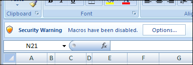
Occasionally, I get calls from clients who don’t understand why their Excel file isn’t working. They’re clicking buttons, or selecting from drop down lists, but none of the usual magic is happening. Is the file broken?


 Last week, I posted Bob Ryan’s Excel macro for