There are lots of different ways to count things in Excel – maybe you need to count the numbers in a column, or all the data, or just the blank cells. Fortunately, there is a function for each of those:
COUNT
COUNTA
COUNTBLANK
For example, to count the blank cells in the range A1:A5, use the following formula in cell A7:
=COUNTBLANK(A1:A5)
More Complicated Counting
If you have more complicated things that you need to count, there are other functions to do the job:
COUNTIF
COUNTIFS
SUBTOTAL
AGGREGATE
For example, to count only the visible numbers, after filtering and/or manually hiding rows in a list, use a SUBTOTAL formula. This example uses 102 as the second argument, so it counts numbers only, in the visible rows (filtered or manually hidden).
=SUBTOTAL(102,B2:B10)
In the screen shot below, there are 5 visible numbers in cells B2:B10, and that is the result in cell B15, where the SUBTOTAL function is used.
The COUNT function, used in cell B12 in the screen shot below, returns 8 – it counts numbers in the hidden rows too.
Watch the Slide Show
To see a quick overview of 7 ways to count in Excel, you can watch this short slide show. It also contains a video on using the COUNTIFS function. You can see more examples on my Excel Count Functions page, and download the sample file.
Count Specific Items With COUNTIF Function
This video shows how to use the COUNTIF function to count cells that
contain a specific string of text, such as “Pen”.
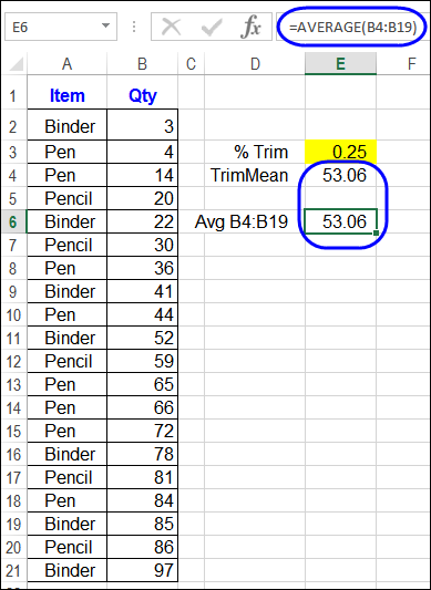
From what I’ve seen in workbooks over the years, SUM is the most frequently used Excel function, and AVERAGE is the runner-up. Would you agree, or do you see other functions used more often than those two?
This Sunday is Super Bowl XLIX – the last one that will start with “XL”. Next year, it will be Super Bowl L – that doesn’t exactly roll off the tongue!
In 2011, I showed how you can use the ROMAN function in Excel, to change a number into a Roman numeral. That year, they were playing for the 45th time, which was XLV.
=ROMAN(A2)
Other Football Functions
There are other Excel functions that sound like they could be used in a football game. Here are a few, and I’m sure you can think of others:
CONVERT
RECEIVE
YIELD
SUBSTITUTE
ISREF
Okay, that last one was a bit of a stretch, but I’ll allow it. What functions did I miss?
Close Football Games
While you wait for the game to start, you can look back at some historic games, with the data that Kevin Lehrbass compiled in an Excel file. You can download Kevin’s workbook, which contains enough data to entertain you for a couple of days, while you try to decide which was the closest game.
Did Kevin think of all the factors that make a football game close, and exciting to watch?
You can even select a couple of Super Bowls, and compare them. Have fun, and enjoy Sunday’s game!
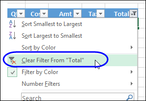
If you’ve highlighted cells with conditional formatting, what’s a quick way to delete the rows those cells are in? Someone asked that question on one of my old blog posts last week. That article showed how to use the Find command, to get a list of cells that contain a specific word. Then, delete the rows for those cells.
It’s a handy trick, but won’t work to select cells that are colored with conditional formatting.
Today’s challenge is to count how many guests stayed at a hotel, in a specific date range, based on the guest arrival and departure dates.
Find Specific Dates
In previous examples, we’ve seen how to check if a specific date falls within a date range. For example, if you have a list of orders, you can use SUMIF or SUMIFS, to add up all the orders between a start and end date. You can see the written instructions for this on my website.
Guest Visits
It is a little trickier to count hotel guests though, because the booking table only shows the guest arrival and departure dates. We have to use those dates, to see if any part of a guest’s visit overlapped our date range.
For this report, we want the number of guest who were in the hotel during the reporting period of December 7th to 9th. I’ve highlighted the records that should be included, when we create a formula to count the guests.
When Did the Guest Leave?
To calculate if the guest’s visit was within the date range, we’ll start with two short formulas.
The first formula will check the guest’s departure date – was it on or after the start of our date range? (If they left before the date range started, they won’t be counted)
The report start date is in cell C3, and guest’s departure date is in cell C6, so the formula is:
=C6>=$C$3
The first 5 guests all left before December 7th, so the result in those rows is FALSE.
When Did the Guest Arrive?
The second formula will check the guest’s arrival date – was it on or before the end of our date range? (If they arrived after the date range ended, they won’t be counted)
The report start date is in cell D3, and guest’s arrival date is in cell B6, so the formula is:
=B6<=$D$3
Guest #11 arrived on December 10, and that is after the report end date of December 9th, so the result in that row is FALSE.
Both Results TRUE
If the result of both formulas is TRUE, then the guest stayed at the hotel during the reporting period:
they arrived on or before December 9th
they departed on or after December 7th
We’ll use a SUMIFS formula to check those two columns, and sum then number of guests in column E. I’ve changed the column headings in F and G, to Dep Check and Arr Check.
The result is 11, and that matches the total when the numbers are selected in the manually highlighted rows. You can see that automatic calculation in the Status Bar.
Download the Sample File
To see how the formulas work, you can download the sample file from my Contextures website. On the Excel Sample Files page, go to the Functions section, and look for FN0036 – Count Hotel Guests in Date Range.
The zipped file is in xlsx format, and does not contain macros. It also has another, more complex, example of counting in a date range. Guests are counted by their hotel loyalty program level, and the number of nights booked in the date range is also calculated.
Video: Count Numbers in a Range – COUNTIFS
Using a simpler example, this video shows how to use the COUNTIFS function to count cells based on a range of numbers.
The minimum and maximum numbers are entered on the worksheet, so it’s easy to change the number range, when needed.
Last week, I heard from someone who was having a problem sorting some numbers in Excel. He sent me a small sample file that showed a few of the dates and numbers that just wouldn’t sort correctly.
My first guess was that the data had been copied from a website – that can cause some strange behaviour, when you paste it into Excel. A quick check with the COUNT and COUNTA functions showed that none of the values in cells C3:C6 were real numbers – they were text.
Last week, I was creating an Excel file with sample data, to use for a few experiments. But don’t worry, they weren’t mad-scientist-type experiments – I was doing Power Pivot experiments, and needed some data to play with.
I needed 2 types of data:
Numbers: sample test scores in one column
Text: random Region names and Gender in other columns.
When you try to use the Top 10 filter, on a list that already has some filters applied, the results probably won’t be what you want. The Top 10 feature ignores the filters on other columns, and just returns values that are in the overall Top 10.
Recently, I showed a workaround for that problem in this blog post: Top Ten Values in Filtered Rows. In that example, I added a new column, and used the SUBTOTAL function to show the value, then filtered that new column. Hidden rows would have a value of zero, thanks to the SUBTOTAL function, so they wouldn’t be included in the ranking.
Thanks to AlexJ for suggesting a great use for the REPT function – setting a minimum row height. He uses this technique to add a bit of spacing in his tables, so they’re easier to read.
You can watch the steps in this video (or watch it on YouTube), and the step-by-step instructions are below the video.
Add Space in an Excel List
For example, here is my To Do list, with a few items to work on, around the house. Most of the Task Descriptions are short, and fit in a single line.