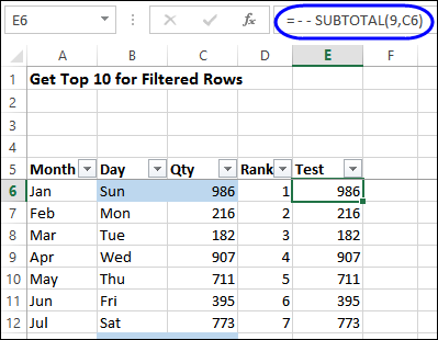
When you try to use the Top 10 filter, on a list that already has some filters applied, the results probably won’t be what you want. The Top 10 feature ignores the filters on other columns, and just returns values that are in the overall Top 10.
Recently, I showed a workaround for that problem in this blog post: Top Ten Values in Filtered Rows. In that example, I added a new column, and used the SUBTOTAL function to show the value, then filtered that new column. Hidden rows would have a value of zero, thanks to the SUBTOTAL function, so they wouldn’t be included in the ranking.

Top 5 for Advanced Filter Results
Last week, someone asked how to do something similar with an Advanced Filter – for products sold after a specific date, which orders had the top 5 amounts?
An Advance Filter is a little harder to use than an AutoFilter, but it has some advantages:
- You can filter in place, or send the results to a different location – even to a different sheet
- Instead of adding a new column, with extra formulas that might slow down the workbook’s calculation, you just need to add a few formulas at the top of the sheet
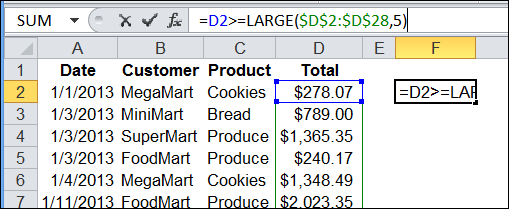
Unlike AutoFilter, the Advanced Filter doesn’t have a built-in Top 10 feature, but you can use the LARGE function in the criteria range, to find rows with the highest values. So, if we just wanted to find the top 5 orders overall, we would use this formula in the criteria range, if the first order amount is in cell D2:
=D2>=LARGE($D$2:$D$28,5)
The formula checks to see if each Total is greater than or equal to the fifth largest number in the list of orders.

Largest Amount After a Specific Date
In this filter, we don’t want to find the 5th largest amount overall – we want to find the fifth largest amount after a specific date. So, instead of a simple LARGE formula, we need a LARGE IF, similar to the MAX IF formula that we’ve created before.
To keep the criteria row visible, I moved the data down one row, so the headings are in row 2. Then, I set up some formulas, that will be used in the Advanced Filter criteria.

H2: The date to be used as the starting date for the filter results
I2: The number of top records to return
K2: A formula that calculates the number of records after the start date
=COUNTIF($A$3:$A$29,”>=” & $H$2)
M2: LARGE IF formula calculates 5th largest Total for orders on or after the start date
=LARGE(IF($A$3:$A$29>=$H$2,$D$3:$D$29),MIN($K$2,$I$2))
- The LARGE function returns the fifth largest value in the range D3:D29, for dates on or after the start date.
- This formula is arrayed entered (Ctrl+Shift+Enter)
- If there are fewer records than the Top # requested, the lower number is used — MIN($K$2,$I$2)
Create the Criteria Range
After the supporting formulas are built, you can create the criteria range for the Advanced Filter.

The criteria cell will contain a formula, so the heading cell is left blank.
F1: Criteria Heading — Leave blank
F2: Criteria: =AND(A3>=$H$2,D3>=$M$2)
In cell F2, the criteria formula checks two things:
- Is the date in cell A3 greater than or equal to the starting date in cell H3?
- Is the amount in cell D3 greater than or equal to the minimum total that is calculated in cell M2 ?
Run the Advanced Filter
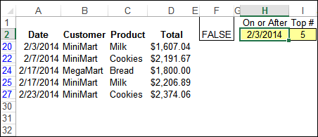
When you run the Advanced Filter, the result is a list of the 5 orders sold on or after February 3rd, with the 5 largest totals. I filtered the list in place, but you could send the results to a different location.

Download the Sample File
To see how this filter works, you can download the Advanced Filter sample file from my website. The file also has an example for finding the highest totals within a specific date range – between a specific start and end date.
Video: Filter Data to a Different Sheet
One of the many useful things that an Advanced Filter can do is copy data to a different sheet, without using a macro. You can see the steps in this video.
The video transcript is below the video.
More Excel Filter Examples
Send Excel Data to Another Sheet
Advanced Filter Criteria Slicers
_________________
Video Transcript
In Excel, you can use an Advanced Filter to pull data from a table and put it somewhere else in the workbook, either on the same sheet or a different sheet.
In this example, we have a list of orders and we would like to pull the orders with the highest totals and put them on a different sheet in the workbook. I would like to get the date and the customer for each of the high priced orders.
Criteria Area
Back on the Orders sheet, I’ve started a criteria area here. I’m using total, which is the column where the order amount is in the main table. That’s the criteria heading, and below that I’m going to enter my criterion, which is greater than 1500.
I only want orders where the total is greater than 1500. I’m not putting dollar signs in here. It’s just the number that I wanted to check.
We want to pull orders onto a different worksheet. In this case, we have to start on this destination worksheet, and I want to stay away from the cells near the heading. So, I’m just going to click a cell somewhere in an empty area of the worksheet.
Start Filter
To start the filter on the ribbon, I’ll go to the Data tab and click Advanced. In the Advanced Filter dialog, I’m going to select Copy to Another Location.
The List range is my main table. So, I’ll click here, then go to the Orders sheet and select the entire table, including the headings. That’s entered as the list range.
My Criteria range, I’ll click in that cell. Go back to the Orders sheet where I created my criteria range and select the heading cell and the criteria cell below that.
For CopyTo, this is where I want the data to end up. I’ll click here and select my two heading cells on the TopOrders sheet and I’ll click OK, and there are the 3 orders where the total is higher than 1500.
If we look back, we can see 1, 2, 3 orders, and those have been copied automatically to the other worksheet using an Advanced Filter.
___________________
