
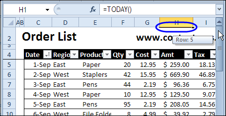
If you want to scroll down the worksheet, and lock the heading rows in place, so they’re always visible, you can use the Freeze Panes command. Be careful though, or you might end up with hidden rows that you can’t get to.
Category: Excel Archive
Tips and tutorials for older versions of Excel
Freeze Panes Disappear in Excel
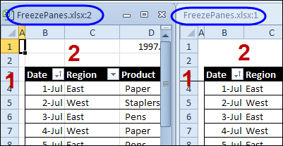
You spend time setting up your worksheets exactly the way you want them – the headings are frozen at the top of the screen, gridlines are turned off, and a few other customizations are made. Beautiful!
Filter Excel Data Onto Multiple Sheets
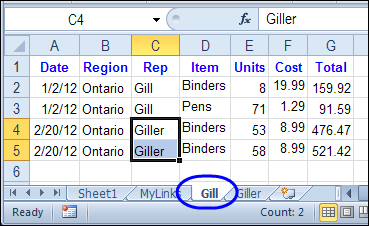
There is a sample Excel file on my Contextures website that has a list of orders, and sales rep names.
It has a macro to filter Excel data onto multiple sheets. You can click a button, and a sheet is created for each sales rep, with that person’s orders.
Excel Power Utility Pack Sale Phase 2
This product is no longer available.
For the latest Excel courses, Excel books and Excel tools, go to the Debra’s Excel Picks page, on my Contextures website

Excel Power Utility Pack Sale
This product is no longer available.
For the latest Excel courses, Excel books and Excel tools, go to the Debra’s Excel Picks page, on my Contextures website
Filter Pivot Charts in Excel 2010
In Excel 2007, there was a PivotChart Filter Pane, and you had to open that if you wanted to filter the pivot chart. Things have improved in Excel 2010, and the PivotChart Filter Pane is gone.
PivotPower Add-in Update
Long ago, when many of the pivot table features were hidden away in obscure menu and dialog boxes, I created the PivotPower add-in. It makes it easy to do pivot table tasks, such as:
- change the summary function for all the data fields from Count to Sum,
- reset the field captions,
- protect the pivot table layout,
- and many other tasks
When you install PivotPower, it adds a a drop down list on the Add-ins tab of the Excel Ribbon, or a menu on the menu bar, in older versions of Excel.

Latest PivotPower Update
In the latest version of PivotPower, most of the commands will only affect the selected pivot table.
For example, if there are two pivot tables on the worksheet, select a cell in one pivot table, before using the COUNT All Data command. The data fields in the selected pivot table will change.

If the active cell is not in a pivot table, all pivot tables on the active sheet will be affected when you run the command. In the screen shot below, a cell between the pivot tables is selected.
When the SUM All Data command is selected, both pivot tables will be changed.

PivotPower Fix
This version of PivotPower also has a fix. In the previous version, if you selected the AVERAGE All Data command, the Data labels changed, and stayed as “Avg” even if you selected a different summary function.
That problem is corrected in this version.
Download the PivotPower Add-in
You can read more about the PivotPower features, and how to install the add-in, on the PivotPower page on the Contextures website.
If you use the PivotPower add-in, and notice anything that should be fixed, please let me know!
___________
Excel Advanced Filter Update
Here’s the final video update for this week — Automatically Copy Excel Data to Another Sheet. This video now shows the steps in Excel 2010 or Excel 2007, instead of Excel 2003.
To wrap up this week of updates, here are links to a few of my previous Excel Advanced Filter articles and posts. You probably know all the basics, but maybe you’ve missed a few of these tips and tricks.
- Click a Map To Filter Excel Data – set up an Excel workbook so you can click on a map of the USA, and see a list of fictional doctors in the state that you selected.
- Excel Advanced Filter Complex Criteria – see examples of criteria you can use when setting up an advanced filter
- Create New Sheets from Filtered List – a macro uses an Advanced Filter to create a separate sheet of orders for each sales rep visible in a filtered list
Note: Remember — the 30 Excel Functions in 30 Days challenge starts January 2nd. See you then!
Watch the Excel 2010 Advance Filter Video
See how to automatically copy data to a different worksheet, with an Advanced Filter, in Excel 2010 or Excel 2007.
There is a full transcript after the video.
Video Transcript
In Excel, you can use an Advanced Filter to pull data from a table and put it somewhere else in the workbook, either on the same sheet or a different sheet.
In this example, we have a list of orders and we would like to pull the orders with the highest totals and put them on a different sheet in the workbook. I would like to get the date and the customer for each of the high priced orders.
Criteria Area
Back on the Orders sheet, I’ve started a criteria area here. I’m using total, which is the column where the order amount is in the main table. That’s the criteria heading, and below that I’m going to enter my criterion, which is greater than 1500.
I only want orders where the total is greater than 1500. I’m not putting dollar signs in here. It’s just the number that I wanted to check.
We want to pull orders onto a different worksheet. In this case, we have to start on this destination worksheet, and I want to stay away from the cells near the heading. So, I’m just going to click a cell somewhere in an empty area of the worksheet.
Start Filter
To start the filter on the ribbon, I’ll go to the Data tab and click Advanced. In the Advanced Filter dialog, I’m going to select Copy to Another Location.
The List range is my main table. So, I’ll click here, then go to the Orders sheet and select the entire table, including the headings. That’s entered as the list range.
My Criteria range, I’ll click in that cell. Go back to the Orders sheet where I created my criteria range and select the heading cell and the criteria cell below that.
For CopyTo, this is where I want the data to end up. I’ll click here and select my two heading cells on the TopOrders sheet and I’ll click OK, and there are the 3 orders where the total is higher than 1500.
If we look back, we can see 1, 2, 3 orders, and those have been copied automatically to the other worksheet using an Advanced Filter.
_________________
Excel Conditional Formatting Update
The holidays are a great time to catch up on tasks. I’ve updated another popular Excel video — Colour a Row Based on a Cell Value in Excel.
To continue the conditional formatting theme, here are a few articles that you might have missed, when they were originally posted.
- Highlight Weekend Dates in Excel – To make it easier to keep track of weekends in Excel, you can use conditional formatting to highlight the rows where the date is a Saturday or Sunday.
- Excel Conditional Formatting – Data Bars – In Excel 2007 and Excel 2010, you can use conditional formatting to add data bars to cells. This makes it easy to visually compare the list of numbers, just as you would in a bar chart.
- Highlight Lottery Numbers with Conditional Formatting – If you win the big draw, you’ll be sure to notice, if you use Excel to highlight the winning numbers.
Watch the Conditional Formatting Video
Watch this short video to see how to colour a row based on a cell value in Excel.
There is a full transcript following the video.
Video Transcript:
With Excel’s conditional formatting, you can easily highlight a cell if it’s over or under a certain value, or if it meets a value that you’ve set.
But in some cases, instead of just a single cell, you might like to highlight a whole row in a table, if one of the cells in that row is over a certain number or under.
In this case, we would like to highlight each row in this list if the number of units sold is greater than 75.
So to do that, I’m going to select all of the rows, all of the columns in each row. So I’ve selected from A2 down to D10.
On the Ribbon, on the Home tab, I’ll click Conditional Formatting, and none of these preset rules will do exactly what I want. So I’m going down to New Rule, and in here I’ll select a formula.
So I’m going to use a formula to determine how to color each row.
When I click that, there’s a spot where I can put the formula.
I want to, in each row, look at the value that’s in column B. So I’ll type =
And we want, from every column, we want to look at column B. So we have to lock that cell. We don’t want it to be relative, we want it to be absolute.
So type a $ to lock that in. And then B.
And we want, in this case, the active cell we can see is white, where the other cells are highlighted with blue.
We can see that, in the name box, A2 is showing up. So that’s the active cell, so the active row is 2. So I’m going to type 2 here.
We’re going to check what’s in B2 and see if it’s greater than 75. So that’s our test.
And if it is greater than 75, we want to format it. So I’ll click Format and I’ll choose a fill color, maybe a blue color and click OK, and click OK again.
And now, any row where the number of units is greater than 75, all four cells in that row are colored blue.
______________
How to Customize the Excel Data Entry Form
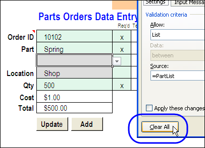
I’ve posted a few versions of the Excel Worksheet Data Entry Form, starting with the original version that Dave Peterson created. Thanks for your comments and suggestions, which give me ideas for enhancing it.
Continue reading “How to Customize the Excel Data Entry Form”