
It’s August already! How did that happen? Did you know that August is not only a month name, it’s an adjective that means “inspiring reverence and admiration; venerable, impressive”. In Excel, it’s also impressive to know how to use array formulas.
Category: Excel Archive
Tips and tutorials for older versions of Excel
Excel Charting Utility Giveaway
Last week, you had a chance to win John Walkenbach’s new book – 101 Excel 2013 Tips, Tricks & Timesavers, thanks to Katie Mohr at Wiley. Thanks for all your comments – those were great tips!
Remove Picture Background and Excel Book Giveaway
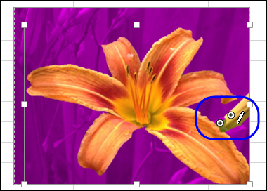
Do you ever put a picture or clip art on a spreadsheet? I don’t use them very often, but occasionally I’ll add a small picture on an instruction worksheet, or insert a company logo on a printable form.
Continue reading “Remove Picture Background and Excel Book Giveaway”
Missing Drop Down Arrows in Excel 2013
You can create drop down lists on a worksheet with Excel’s data validation feature, and they make data entry much easier – usually! Sometimes things go wrong though, like missing drop down arrows in Excel 2013. Have you seen that problem?
See Formula Results in an Excel Data Table
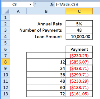
Do you ever use the Data Table feature in Excel? It’s one of the “What-if Analysis” tools, found on the Ribbon’s Data tab, along with Scenario Manager, and Goal Seek.
You can experiment with one or two variables in a formula, and see formula results in an Excel Data Table, in a compact layout.
Continue reading “See Formula Results in an Excel Data Table”
Create Excel Table With Specific Style
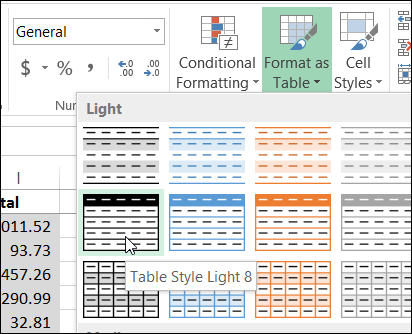
When you create a named Excel table with the Table command on the Ribbon’s Insert tab, the table retains any formatting that it currently has, and the default Table Style is applied.
Midnight Times Missing in Excel Worksheet
Last week, I was working on a client’s time sheet file, and noticed something strange. The worksheet was used to record shift start and end times, and I was testing the calculations, to make sure that everything was working correctly.
Time Past Midnight
Shifts that run past midnight can cause problems, so I tested that scenario, and I also tested shifts that started at midnight. I wanted to be sure that everyone would get all the pay they were entitled to!
In column D, I calculated the hours worked, by subtracting the start time from the end time, and adding 1 to the end time, if it was in the next day. Here is the formula in cell D2:
=(C2+IF(OR(C2=0,C2<B2),1,0)-B2)*24

Missing Midnight
The calculations were working well, but the cells where I had entered a midnight time appeared empty.
Fortunately, the calculations still worked, even with the missing start times.
I know that midnight is a favourite time for mysterious things to happen in horror movies, but was my worksheet haunted? Was this an early Halloween prank?

Hidden Zeros
Finally, I realized that someone had formatted the worksheet to hide the zeros. And, if your worksheet is formatted to hide zeros, the midnight times won’t show, because they are equal to zero – 0:00
To fix the problem, I turned the Show Zeros setting back on, and all the midnight times came out of hiding.
To show zeros on a worksheet
Here are the steps I followed, to show the worksheet zeros:
- At the top left of the Excel window, click the File tab, then click Options.
- At the left, click the Advanced category
- Then, scroll down, and in the Display options for this worksheet, add a check mark to “Show a zero in cells that have zero value”
- Click OK to close the Options window.

Unhide Your Zeros
I had forgotten all about this problem, until someone left a comment on my blog yesterday, asking why the midnight times weren’t showing in her worksheet.
At least I’m not the only one who has had this mysterious problem, and if it has happened to you, I hope this tip helps.
It’s not one of Excel’s most complicated problems, but it’s the little things that can drive you crazy. 😉
____________________________
Conditional Formatting Updates in Excel 2010
If you’re upgrading to Excel 2010, you’ve probably noticed that the Conditional Formatting feature has changed quite a bit.
Now you can apply more than 3 rules, and there are fancy features like data bars and icon sets.

Intro to Conditional Formatting
On my Contextures site, I’ve updated my Intro to Conditional Formatting page, to show Excel 2010 instructions. I’ve also made a new video to show the steps n the new version of Excel.
Note: If you’re looking for Excel 2003 instructions, they’ve been moved to this page: Excel 2003 instructions.
Video: Excel Conditional Formatting Rules
To see the steps for creating two conditional formatting rules in Excel 2010, you can watch this short video.
I show how to add conditional formatting rules that colour a cell, to make the high and low values stand out on an Excel worksheet.
You can enter the minimum and maximum values on the worksheet, and edit them there, to make the conditional formatting settings easy to adjust later.
Video: Sort Based on Conditional Format Icon
When you are working with lists in Excel, use the built-in Table feature, to enable sort and filter commands, and other powerful features.
In the table, you can use drop down arrows in the heading cells, to sort and filter the data
If you add conditional formatting icons, or if you color the cell or the font, you can also sort and filter by those colors.
Watch this short video to see the steps for adding cell icons, and sorting by the selected cell’s icon.
To get the Excel sample file, go to the Sorting in Excel page on my Contextures site:
Download the Sample File
To see the sample used in this video, and other conditional formatting examples, you can visit the Conditional Formatting Introduction page.
___________________
PivotPower Free Excel Add-in
Do you use the free Pivot Power add-in that’s available on my Contextures website? I created Pivot Power to make my own work easier to do, and shared it on my website to help you with your pivot table tasks.
It automates some of the features that aren’t built in to an Excel pivot table, and makes some of the buried Excel pivot table features easier to access.
For example, there is a command that changes all the data fields to SUM, which is handy when Excel defaults to COUNT.

Get Free Pivot Power Add-In
Click here to go to the download page for this free add-in is still available, and try it out!
_______________
Create Alternating Shaded Rows on Excel Sheet
If you’re using a named Excel table, you can apply a style that shades alternate rows with colour. In the table shown below, the row shading has two rows of grey followed by one row of white.
To create this table style, I duplicated one of the existing styles, and modified the row shading.

If you don’t want to use a table, or table styles aren’t available in your version of Excel, you can still have shaded rows, by using conditional formatting.
Shade Rows With Conditional Formatting
To shade the rows, we’ll use the MOD function in a conditional formatting formula. To see how it works, we can test the MOD function on the worksheet, in column G.
We want a set of 3 rows – two with shading, and then a row with no colour. With the MOD function, we’ll get the remainder, if the row number is divided by 3.
=MOD(ROW(),3)
The result for each row is shown in column G, and is either 0, 1 or 2.

We can shade rows where the result is 0 or 1, and leave the rows with 2 as no fill colour. To check the result of the MOD function, we can add a formula in column H, to see if it’s less than 2.
=G2<2

If the result is TRUE, we can shade the row. I’ve highlighted the TRUE cells in the screen shot above, to show which rows will be shaded.
Columns G and H were just used to test the formula, so I’ll clear those out, before formatting the cells.
Create a Conditional Formatting Formula
To shade the rows, we’ll combine the MOD function and the test of the results, in a conditional formatting formula.
- Select the cells where you want the banded rows to appear. In this example, cells A2:F9 are selected.
- On the Ribbon’s Home tab, click Conditional Formatting, then click New Rule
- For Rule Type, click on Use a Formula to Determine Which Cells to Format
- For the formula, enter =MOD(ROW(),3)<2
- Click the Format button.
- On the Patterns tab, select a colour for shading – light grey was used in this example
- Click OK, click OK

The selected range has two rows of grey shading, followed by a row with no fill colour.

Make the Shaded Rows Adjustable
In the previous example, the numbers 3 and 2 were typed into the conditional formatting formula. To make the shading adjustable, you could enter the numbers on the worksheet, and then refer to those cells in the formula.
On the worksheet, create an input range for the numbers. In this example, the numbers are entered in J1 and J2, and the sum of those numbers is in J3.

Modify the Formula
To change the conditional formatting formula:
- Select a cell in the range where the conditional formatting rule was applied. In this example, cells A2:F9 are selected.
- On the Ribbon’s Home tab, click Conditional Formatting, then click Manage Rules
- Click on the MOD rule in the list of rules, and click Edit Rule
- Change the formula, so it refers to the grey shading number — $J$1, and the total number — $J$3:
- =MOD(ROW(),$J$3)<$J$1
- Click OK, click OK

Test the Shading
To test the interactive shading formula, change one or both of the numbers in J1:J2. The shading on the worksheet should automatically adjust.
In the screen shot below, the numbers were changed so there is one grey row, followed by 2 rows with no fill.

Watch the Video
To see the steps for creating shaded rows on the worksheet, please watch this short video tutorial.
Download the Sample File
To download the sample file, please visit the Conditional Formatting Examples page on my Contextures website. The Excel 2010 / 2007 sample file contains the interactive example.
______________________________