Last Friday, January 8th, would have been Elvis Presley’s 75th birthday. Sadly, he died in 1977, so he never had a chance to work with Microsoft Excel. Otherwise, he might have sung “A Little Less Concatenation”, instead of “A Little Less Conversation.”
Let it snow! One of the advantages of working from home in Canada, is that you don’t have to go out in rush hour, on snowy days. I can sit in my office, basking in the glow of the computer monitor, mesmerized by the flickering of the modem lights.
But eventually I’ll have to go out to do some shovelling, in the sub-zero temperatures. Later, while thawing out, I’ll create an Excel file, to track the miserable temperature and snowfall accumulation.
A Matter of Degree
We record our temperatures in Celsius, while our neighbours in the USA use a Fahrenheit scale. So, while I’m shivering on a -10°C day, it seems much warmer across the lake, where it’s a balmy 8°F.
I’m sure there are good reasons why the USA didn’t switch to the metric system when Canada did, but for now, we can use Excel to convert the temperatures.
Use Arithmetic
Maybe the temperature in the USA really isn’t as warm as it seems.
To convert the temperature from Fahrenheit to Celsius , you can use this formula:
°C = (°F – 32) x 5/9
If the Fahrenheit temperature is in cell B2, put this formula in cell C2:
=(B2 – 32) * 5/9
When I convert that balmy 8°F, it makes me feel better – it’s actually colder there, at -13°C.
Let Excel Convert It
That formula isn’t too difficult, but it might be hard to remember if your brain is affected by the cold weather. An easier way to convert the temperature is to use Excel’s CONVERT function.
Note: If you’re using Excel 2003, or an earlier version, you’ll need to install the Analysis ToolPak to use the CONVERT function.
Excel CONVERT Function
With the CONVERT function, you refer to the cell that contains the amount that you want to convert. Then you enter the original unit of measurement, and then the new unit of measurement.
We want to convert the value in cell B2, from Celsius (“C”) to Fahrenheit (“F”).
=CONVERT(B2,”C”,”F”)
Later, I can use CONVERT to see how many inches of snow we got, when the weather channel reports the snowfall in centimetres.
Excel Help for CONVERT Units
If you aren’t sure what code to use for each unit of measurement, you can check the list in Excel’s help for the CONVERT function.
Excel Help for CONVERT Units
Now I have to go and figure out how many glasses of wine are in that 750 ml bottle. I think the answer might be – not enough!
Do you have Excel horror stories, that you like to tell around the campfire, to scare your friends?
One of my recent Excel horror stories involves Excel sheet names. I set up a client’s workbook with pre-formatted data entry sheets, so sales managers could plan their annual product promotions.
They would rename the data entry sheets while working, to make it easier to navigate the completed workbook.
Hidden Sheet With Formulas
On a hidden summary sheet in the workbook, I added formulas to calculate the sheet names.
In another column on that sheet, a few Excel INDIRECT function formulas pulled data from specific cells on each data entry sheet, and other formulas created grand totals.
At the front of the workbook, the summary data was displayed in a monthly calendar, for sales managers to review. It was a work of art!
The Scary Phone Call
Everything worked well in testing, so we distributed the files to all the sales managers, and they started filling in their data.
The next day, the phone rang – some of the workbooks were “broken.”
Budget deadlines were looming, and the sales managers with broken files were in a panic. They sent me a couple of problem files, so I could figure out what was wrong.
Summary Sheet Formula Errors
On the Summary sheet, some of the formulas were working correctly, but others showed #REF! errors.
Comparing the good and bad sheets, I couldn’t see any problems with the data that had been entered, at first glance.
Summary Sheet Formula Errors
Sheet Name Apostrophes
Finally, after checking a few of the problem sheets, I spotted a similarity.
All of the problem sheets included an apostrophe in the sheet name!
I removed the apostrophes, and the problem was solved.
All the data showed up in the summary sheets, and the world was in harmony once again.
Note: For the next version of the workbook, I updated the workbook’s Summary sheet formulas, using the Excel SUBSTITUTE function.
Sheet Naming Rules
I hadn’t anticipated that problem, since I never use apostrophes in sheet names. They’re valid characters for a sheet name, but maybe they shouldn’t be.
It’s hard to find the sheet naming rules in Excel’s help, but you may have seen an Excel error message that lists them.
The name can’t be more than 31 characters
You can’t leave the sheet tab blank
Only a few characters are listed as invalid, like the following ones from the error message below:
: \ / ? * [ ]
colon, back slash, forward slash, question mark, asterisk, open square bracket, close square bracket
Apostrophes are okay though!
Excel error message: You typed an invalid name for a sheet or chart”
Sheet Naming Suggestions
In addition to those rules, I have a couple of guidelines of my own.
Use only letters, numbers and underscores in sheet names.
Sometimes I have to use a space character, if a client requests specific sheet names, but I try to avoid it.
For example, I’d use SalesData or Sales_Data, not Sales Data.
And please – don’t use apostrophes!
Use different names for worksheets and named ranges, to avoid confusion.
However, this does NOT work in our sample table, because it stops at the M7, and that’s not an exact match for the lookup value m7.
Case Sensitive INDEX MATCH
The Microsoft article has other sample formulas, including an INDEX MATCH, but they all have the same problem — they stop at the M7 above the m7 value.
Fortunately, a search in Google Groups led me to an array formula posted by my old friend, former Excel MVP Peo Sjoblom.
For our table, Peo’s formula would be this array-entered INDEX, MATCH and EXACT combination:
=INDEX(B1:B6,MATCH(1,--EXACT(A1:A6,D1),0))
Note: To array-enter this formula, type the formula, then press Ctrl+Shift+Enter. Curly brackets will automatically appear at the start and end of the formula.
Case Sensitive Formula – Correct Result
In the screenshot below, the revised formula is entered in cell E1.
Its formula is visible in the Formula bar, and the correct result of 5, is showing in cell E1.
The formula finds an exact, case-sensitive match for the lookup value, m7, that I typed in cell D1
Last week I was testing a client’s workbook, and had filled in all the data entry cells, to make sure everything was working correctly.
Find Data Entry Cells
Before sending the workbook back to my client, I wanted to clear all the data entry cells.
Instead of selecting each cell individually, and clearing it, it would be easier to clear groups of adjacent cells where possible.
However, some cells had formulas, and I didn’t want to accidentally clear any of those.
If the formulas are visible, that would prevent the problem.
See Formulas in Excel 2003
If you’re using Excel 2003, follow these steps to see the formulas on the worksheet:
On the Tools menu, click Options
On the View tab, add a check mark to Formulas.
See Formulas in Excel 2007
If you’re using Excel 2007, follow these steps to see the formulas on the worksheet, instead of the formula results:
Click the Office button, then click Excel Options
Click the Advanced category
In the Display Options for This Worksheet section, add a check mark to
Show formulas in cells instead of their calculated results.
Show or Hide Formulas with a Keyboard Shortcut
The keyboard shortcut to show or hide the formulas is
Ctrl + `
The symbol at the right is an accent grave, and that key is above the Tab key on the my laptop’s keyboard. It might be in a different location on yours
The accent grave looks similar to an apostrophe, but its top leans to the left, instead of being straight up and down.
If you’ve imported data into Excel, you might need to clean it up before you can use it. The video, and written steps below, show how to fill blank cells in Excel to complete a table.
“Help!” said the familiar voice, when I picked up the phone at 10 PM.
“I have a list of orders in an Excel sheet. I want to compare it with the list from last week, and delete all the orders that were in the old list.”
It was my daughter, still at the office, trying to get a pile of work done before the looming deadline. I helped her with a COUNTIF formula, and she was able to leave for home a short time later. Phew!
Find Duplicates With COUNTIF
The first step is to check each OrderID in the new list, to see if it’s also in the old list.
We’ll use a COUNTIF formula to calculate how many times each OrderID is found in the old list. If the count is zero, we know it’s a new order.
Prepare the Worksheets
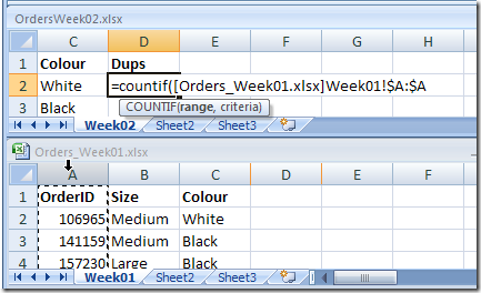
Open both workbooks. Here they’re arranged vertically, so both lists are visible.
two workbooks arranged vertically
In the new workbook, add a column heading, Dups, in cell D1 in this example. This step isn’t required, but keeps things tidier when you try to sort later.
Add COUNTIF Formula
To start the formula, in cell D2, type: =COUNTIF(
Next, we’ll tell Excel where to look for the OrderID. In the old list, click on the column heading for column A, where the Order IDs are listed. That adds a reference with the workbook name, sheet name and column.
=COUNTIF([Orders_Week01.xlsx]Week01!$A:$A
Finally, we’ll tell Excel what we want to look for. Type a comma, then in the new list, click on the OrderID in cell A2.
To complete the formula, type a closing bracket, then press Enter. Here’s the completed formula.
=COUNTIF([Orders_Week01.xlsx]Week01!$A:$A,A2)
Copy the formula down to the last row of data in the new list. There are 1s in some rows and 0s in other rows.
Check Formula Results
We can see that the first three numbers in the new list are also in the old list, and they have been correctly counted as 1.
The next three numbers aren’t in the old list, so their count is zero.
Delete the Duplicates
Now that the new orders are identified with a zero, we can delete the old orders.
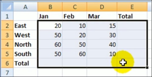
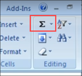
Click in the Dups column heading, and press Ctrl+A, to select the entire range.
On the Ribbon’s Data tab, click the A-Z button, to sort the list in ascending order.
The new items (zeros) will sort to the top of the list, with the old items (ones) at the bottom of the list.
Select all the rows with old items, right-click on a row button in the selected rows, and click Delete.
Finally, to clean up the sheet, delete the Dups column.
Save a copy of the revised file, send it off to your vendor, and go home! (Well that’s how our scenario ended – you might have to stay at work for a few more hours.)
Video: Count Specific Items with COUNTIF
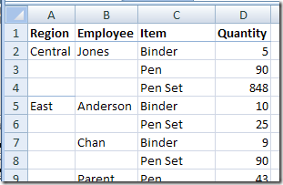
See how to use Excel COUNTIF function to count cells in a list that contain specific words or part of a word. For example, how many orders were for a Pen? How many orders for any kind of pen, such as “Gel Pen”, “Pen” or even a “Pencil”?


 We record our temperatures in Celsius, while our neighbours in the USA use a Fahrenheit scale. So, while I’m shivering on a -10°C day, it seems much warmer across the lake, where it’s a balmy 8°F.