
On Monday, we declared this Excel Advanced Filter Week, in honour of the three filter feeding shark species. Who said Excel wasn’t exciting?
Excel Filter for Blanks: Shark Week
 Last year, we celebrated the Discovery Channel’s Shark Week, by using the LARGE and FLOOR functions.
This year, we’ll pay tribute to the three known species of sharks that are filter feeders, by declaring this Excel Advanced Filter Week.
Yes, we’ll have three fun-filled, action-packed days of Excel filtering fabulousness – one day for each filter feeding shark. Please hold your applause until all three articles have been posted.
Advanced Filter Criteria Range
We’ll kick off the week’s celebrations by filtering rows with missing data (blank cells) to a different worksheet.
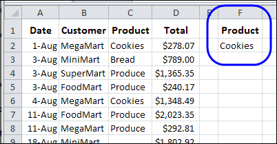
When you’re using an Advanced Filter, usually you would enter a heading, and one or more criteria, in a criteria range, like the one shown below.
In this example, you would be filtering the customer order list for any orders with Cookies as the product.
Blank Cells in Data
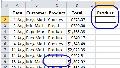
However, if you want to filter orders with a blank cell for Product, you can’t just leave the criteria range blank.
A blank criteria cell is interpreted as “No criteria”, so all the records would pass through the filter. That might be fine for a shark, but not for an Excel report.
Filter for Blanks in Advanced Filter
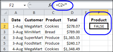
Instead of leaving the criteria cell blank, you can use a formula, to check for empty cells. In this example, the first product data is in cell C2, so the formula is:
=C2=””
The two double quote marks represent an empty string, so if C2 is not blank, the formula result is FALSE.
Only the records that calculate to TRUE would pass through the filter.
Remove the Criteria Range Heading
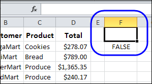
If you’re using a formula in an Advanced Filter criteria range, the heading can’t match any of the source data headings.
You can either clear the heading cell in the criteria range, or type a different heading.
I usually clear the heading cell, because that’s quick and easy!
Run the Advanced Filter
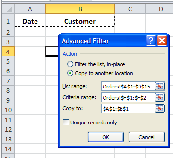
After you set up the criteria range, you can run the Advanced Filter. Remember, if you want the results on a different worksheet, select that destination sheet before you run the filter.
In this example, the filter is started from the Blank Orders sheet, and the list and criteria range are on the Orders sheet.
Download the Advanced Filter Blanks Workbook
To see the sample data, and test the filter, you can download the Advanced Filter for Blanks sample workbook. The file is in Excel 2007 format, and is zipped.
Watch the Advanced Filter for Blanks Video
To see the steps for setting up the criteria range, and running the filter, you can watch this short Excel video tutorial.
___________________
Excel Function Friday: Average Top 10 Scores
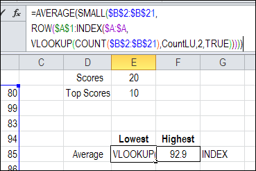
If you have a worksheet with 20 scores listed, how can you calculate an average top 10 scores? And if there are only 11 scores, can the formula automatically adjust, to average just the top 4 scores?
Continue reading “Excel Function Friday: Average Top 10 Scores”
How to Find MIN IF or MAX IF in Excel
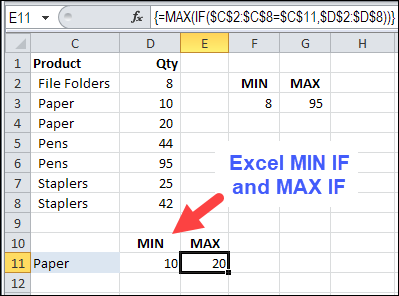
When you were first learning how to use Excel, you quickly discovered the basic Excel functions, like SUM, COUNT, MIN, MAX, and AVERAGE. Now you’re ready for advanced calculations, like how to find MIN IF or MAX IF in Excel.
No Duplicates in Multiple Selection Excel Drop Down
Thanks to an email question from Leslie, I’ve done another variation on the Data Validation Multiple Selection sample.
Leslie is scheduling training courses, and has a table with dates across the top, and course names down the side. One or more of the instructor names can be selected for each training session.
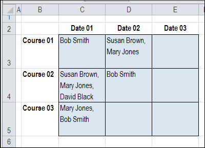
However, Leslie wants to prevent an instructor’s name from being selected twice on the same day. For example, on Date 01, in the screen shot above, Bob Smith and Mary Jones are each booked for 2 courses.
Check for Existing Names
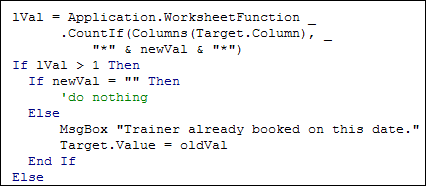
To prevent the names from being selected twice, I changed the code, to include the COUNTIF function.
- After a name is selected, the active column is checked for that name.
- If the name is found, a warning message is shown, and the name is not added in the current cell.
Here is the revised section of the code, with the COUNTIF function:
Testing the Code
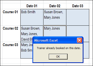
With the revised code, if I try to select a trainer who is already booked, I see this message, and the name is not added.
Download the Sample File
If you’d like to test the Block Duplicates code, you can download the No Duplicates in Multiple Selection Excel Drop Down sample file.
The file is in Excel 2007 format, and is zipped. When you open the file, enable macros, if you want to test the block duplicates feature.
_____________
Make It Easy to Ask Excel Questions
While working with PowerPivot in Excel 2010, I noticed the Ask Questions command on the Ribbon.
When you click that command, your web browser opens, and takes you to the PowerPivot Help forums on the Microsoft website.
That’s a nice feature, if you’re struggling with PowerPivot.

Where Do You Ask Excel Questions?
Why doesn’t Excel have an Ask Questions command? We have questions too! (A moment of silence for the old Excel newsgroups.)
The closest thing that I could find is a Contact Us command, which leads to the Microsoft website.

Microsoft Answers Forum
At the bottom of that page is a link that leads to the general Answers form – not to an Excel related forum. It takes a couple more clicks to get to the Excel section.

Ask Excel Questions
Maybe that Ask Questions command will be in the next version of Excel. Until then, here are links to the Excel help forums on the Microsoft site.
Answers – http://answers.microsoft.com/en-us/office/forum/excel
Technet — http://social.technet.microsoft.com/Forums/en/excel/threads
MSDN (Excel Developers) — http://social.msdn.microsoft.com/Forums/en-US/exceldev/threads
MSDN (VBA) — http://social.msdn.microsoft.com/Forums/en-US/isvvba/threads
There are links to other Excel forums in the following article that I wrote:
- The Excel Newsgroups Disappeared.
_________________
Normalize Data for Excel Pivot Table
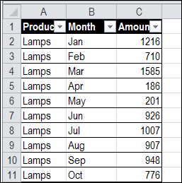
If your Excel data is in monthly columns, like the worksheet shown below, you’ll have trouble setting up a flexible pivot table. Instead of leaving the data like this, see how to normalize data for Excel pivot table setup.
Find Last Row With Excel VBA
 Recently, I complained about having trouble getting Excel VBA to correctly find the last row with data in a column, when using Excel tables. Thanks for the suggestions on solving that problem!
Jim Cone was intrigued by the find last row challenge, and from previous Excel adventures, Jim knew that Excel tables aren’t the only obstacle to finding the last row.
Universal Last Row Function
Jim decided to write a universal LastRow function for a…
- Worksheet
- Range (selection)
- Specific column – in a worksheet or range.
- List/Table
- Filtered data
Last Row in Selection
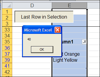
For example, the LastRow function shows that row 40 has the last value in column E, even though that row is hidden by a filter.
How to Find the Last Row
Covered with dust, and bits of Excel VBA code, Jim has finally emerged from his basement workshop. He sent me his Find Last Row sample workbook, which you can download at the link below.
Here’s what Jim had to say about writing the code:
- The (A) Find function and (B) Iteration of each column have advantages and disadvantages.
- The find function is faster, works on List/Tables but fails on a filtered range and occasionally throws up an unexpected error.
- The iteration method seems to be generally reliable but fails on both Lists/Tables and filtered ranges.
And Jim added more details:
- In the past, I’ve used different pieces of code to find the last row as different circumstances dictate, but finally decided to put together a one size fits all answer. The following code is what I came up with.
- Note that it is actually two functions (both are required).
- Use of the second function avoids a compile error in Excel versions prior to the 2003 version.
- The approach is to search using find and switch to iteration if an error occurs.
Thanks Jim!
Download the Sample Workbook
To see Jim Cone’s Excel VBA code, you can download the Find Last Row in a Column sample workbook. The file is in Excel 2003 format, and zipped. Enable macros when opening the file, if you want to test the code.
Jim has added a few Excel tables to the worksheet, which you’ll see in Excel 2007 and Excel 2010. In Excel 2003, those will appear as lists.
Click the button on the worksheet, to find the last row with data in the current selection.
Or, you can modify the “DoesItWork” sub, so it will find the last row on a worksheet or specific column.
________________
Save Time When Saving Excel Files
Last week, Seth Godin recommended hiring a geek to help you save an hour a day.
Well, you’re a geek, so you don’t have to hire one! Just pay attention as you run through your morning office routine, and answer this question:
- What can you change about your Excel habits, to save an hour a day, or even a few minutes?
Then, make the change.
Doing Steps Manually
Every morning, I follow these steps:
- download some website statistics to Excel,
- crunch the numbers, and
- save the raw data file.
Fortunately, I have a macro that does the first 2 steps. For some reason, I was doing the last step manually. Don’t ask me why.
Excel is a bit slow when opening the Save As dialog box, so that final step was taking 30-60 seconds. Not a huge productivity drain, but why do something manually, if it can be easily automated?
Make It Automated
To get rid of that manual step, I added a few lines of code to the existing macro. The Excel VBA code saves a copy of the active workbook, into the Backup folder, and adds the previous day’s date to the file name.
It only took me a couple of minutes to add the code, so the time invested was quickly repaid. Now I just have another 59 minutes to trim!
Macro Code to Save Daily File
'------
Sub SaveDailyData()
Dim wbData As Workbook
Dim strDir As String
Dim strName As String
Dim strExt As String
Set wbData = ActiveWorkbook
strDir = "C:\Backups"
strName = "DailyData_" & Format(Date - 1, "yyyymmdd")
strExt = ".xls"
wbData.SaveCopyAs strDir & strName & strExt
wbData.Close SaveChanges:=False
End Sub

___________
Excel CONVERT Function Made Easy
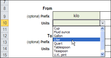
Do you ever use the Excel CONVERT function? Or, do you avoid that function, because you can’t remember all the measurement unit codes?
For example, the formula =CONVERT(10,”klt”,”gal”) will convert 10 kilolitres to 2,641.7205 gallons – if you get those codes right.
You might be able to remember lt and gal, but probably not many of the other codes.