
I’m working on some pricing reports for a client, and one of the requests was for a Pocket Price Waterfall chart. I hadn’t made one of those before, and fortunately the client sent me a sketch of the chart that they wanted.
Move ListBox Items In Excel UserForm
Last week, we saw how to move items from one listbox to another on an Excel worksheet.
Now I’ve added a page on the Contextures website, with similar instructions for listboxes on an Excel UserForm.
Thanks to Dave Peterson, who provided both sets of sample code.
ListBoxes in Excel UserForm
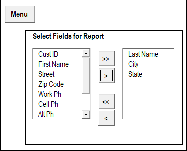
In the screen shot below, there is an Excel UserForm with two ListBoxes, and four command buttons, down the centre.
- The buttons with 2 arrows move ALL items from one list to the other, in the direction that the arrows are pointing
- The buttons with 1 arrow move the SELECTED items from one list to the other, in the direction that the arrow is pointing

Download the Move Listbox Items Sample File
To see the code, and test the ListBox move items code for a UserForm, you can download the ListBox UserForm Move Items sample workbook.
The file is in Excel 2007 format, and is zipped. It contains macros, so enable them if you want to test the code.
Related Excel VBA Tutorials
If you’re looking for a fun and exciting way to fill your holiday Monday, here are links to a few other UserForm and Excel VBA tutorials on my Contextures website:
Create an Excel UserForm Video
Excel VBA Edit Your Recorded Macro
______________________
Holiday Weekend Flags in Excel

Happy Canada Day! I made a couple of holiday weekend flags in Excel, to help you celebrate.
Move Excel Listbox Items
To select specific items from a long list, you can create 2 ListBoxes on a worksheet.
Then, use arrow buttons to move all the items from one list to the other, or move selected items only.
ListBoxes on Worksheet
In the screen shot below, there are 2 ListBoxes, and 4 buttons with arrows, on a worksheet named CreateRpt.
- In the ListBox at the left, you can select one or more items that you’d like in a report.
- Then, click the 2nd button, with one arrow that point to the right.
- The selected items will move to the ListBox on the right.
OR
- You could click the. top button, to move all the items to the right-hand ListBox.
Items List on Worksheet
When you get started, the list at the left is filled with items. Those items come from a named range, on a worksheet named Admin.
You could modify that list, to include the items that you need in your ListBox.

Use the ListBoxes
In the sample file that you can download, there is a Menu worksheet, with a navigation button, “Select Report Items”.
Click that button to go to the CreateRpt worksheet, where the ListBoxes are located.

Macro Runs Automatically
When the CreateRpt sheet is activated, an event procedure (macro) runs automatically.
The VBA code in that event procedure does the following steps:
- Clears both ListBoxes
- Adds all items from worksheet list, in ListBox at the left
Back to Menu Sheet
On the CreateRpt sheet, there is another navigation button, “Menu”, at the top left of the sheet.
Click that button, and a macro runs, to take you back to the Menu sheet.
Navigation Button Macros
The two navigation buttons run simple macros, and the VBA code is shown below.
First, here is the code that the Menu button runs:
Sub GoMenu()
Worksheets("Menu").Activate
End Sub
Next, here is the code that the Select Report Items button runs:
Sub GoRpt()
Worksheets("CreateRpt").Activate
End Sub
Read the Detailed Instructions
Thanks to Dave Peterson, who sent me the instructions and sample code for moving listbox items.
To see the details on how this technique works, visit the Excel VBA Move Listbox Items page on the Contextures website.
The tutorial shows, step by step, how to set up the worksheets, add the ListBoxes, and create the named ranges.
It also shows all of Dave’s sample code, for moving the items between the ListBoxes.
Download the Move Listbox Items Sample File
To see the code, and test the Listbox move items code, you can download the Listbox Move Items sample workbook.
The file is in Excel 2007 format, and is zipped. It contains macros, so enable them if you want to test the code.
Video: Move Listbox Items on Worksheet
To see the steps to create the Listbox example, you can watch this Excel video tutorial.
______________
Quickly Find Excel Ribbon Commands
If you have been using the Ribbon in Excel 2007 or Excel 2010 for a while, you can probably find most of the commands that you need. It’s those infrequently used commands that cause the problems. You knew where they were on the old menu bar, but where the heck are they on the Ribbon?
[Update: This Microsoft download is no longer available]
The Office Labs people at Microsoft have taken pity on our poor, fumbling fingers, and come up with a solution – the Search Commands add-in. This free tool lets you type the name of a command, and magically find it. Think of all the time that you’ll save!
For now, at least, the add-in is only available in English, and works in Word, Excel and PowerPoint. It requires Windows XP, or later, operating system.
Download the Search Commands Add-In
To install the Search Commands add-in, go to the download page on the Microsoft site.
Optional – Click on the plus signs, to see
- Details
- System Requirements
- Install Instructions
Then, click on the Download button, to get the file. Next, run the downloaded file, to install the add-in.
Search for Commands
After you run the setup program, to install the add-in, a Search Commands tab automatically appears on the Ribbon.

- In the Search box, at the left end of the Ribbon, type the name of the command that you want to use. For example, if you can’t find the command to protect the worksheet, type “Protect” or “Protect Sheet”.
- Click the magnifying glass symbol, to start the search
- One or more commands that match your search term will appear in the search results section, to the right of the search box.

If there are several commands that match your search words, you might need to use the Previous and Next buttons to scroll through the list of commands.
For example, if you type “Protect”, instead of “Protect Sheet”, there are 16 commands found, shown on 2 pages.

Use the Search Results
If the search results include the command that you were looking for, just click on it, to run that command. Quick and easy!
And to find out where that command lives on the Ribbon, point to the command, before you click it. The popup description shows the location of the command, by listing the Tab, command group, and command name.

It’s funny – I didn’t realize that the Protect Sheet command was also on the Home tab. I expected it to point to the command on the Review tab. It must look for the first instance of the command in the Ribbon tabs.
Also, the location description doesn’t mention that you have to click the Format command, to see the Protect Sheet command, so you might need to do a bit of searching, to find the exact location.

Commands Not in the Ribbon
Another nice feature of the Search Commands add-in is that it even finds some commands that aren’t in the Ribbon.
For example, if you type Pivot, it shows the PivotTable and PivotChart Wizard command.

Room for Improvement
The Search Commands add-in is a work in progress, so it’s not perfect yet.
- It should have full descriptions of the location, as mentioned in the Protect Sheet example above.
- The Search Commands tab doesn’t shrink, when you make the Excel window narrower, like other tabs do.
- Include settings that are in the Excel Options window, like hiding zeros on the worksheet, or changing to R1C1 Reference Style.
What features would you like to see in the add-in?
Customize Excel Ribbon Tab
You can also customize the Excel Ribbon, by moving or removing the groups on a default Ribbon tab. In this video, see how to move groups on the Data tab, so the tools that are used most often are in the middle of the tab, and easier to reach.
Related Articles
Excel Ribbon — Getting Started
__________________
Last Row Incorrect With Excel Table
When you’re working with Excel VBA, you might want find the last row with data, so you can paste new data in the row below that.
The following code works up from the last row on the worksheet, until it hits a cell with data. It’s like using the End key and Up arrow, to manually move from the bottom of the worksheet.
Sub GetLastRow()
Dim ws As Worksheet
Dim lRow As Long
Set ws = ActiveSheet
lRow = ws.Cells(Rows.Count, 1).End(xlUp).Row
MsgBox lRow
End Sub
In the sample sheet, the last data in column A is in row 10, and that’s the result when running the code.

Unexpected Result
This week, I was using similar code in a client’s workbook, to find the last row of data. The data was in a named Excel table, and the last couple of rows in the table were blank. I wanted to find the last row with data, so I could change the table definition, to end at that last row.
When I used the same Excel VBA code, the last row wasn’t what I expected – it found the last row in the named table, even though that row was empty.

I’m sure that information is helpful in some situations, but it sure wasn’t going to help me resize the table!
My Last Row Workaround
There might be a more sophisticated solution to this problem, but I added a line of code to resize the table, so it ends at row 2.
Then, the code found the correct last row of data, and resize the table to end at that row.
Sub ResizeTheTable()
Dim ws As Worksheet
Dim lRow As Long
Set ws = ActiveSheet
ws.ListObjects(1).Resize ws.Range("$A$1:$H$2")
lRow = ws.Cells(Rows.Count, 1).End(xlUp).Row
ws.ListObjects(1).Resize ws.Range("$A$1:$H$" & lRow)
MsgBox lRow
End Sub
That fixed the problem, and the table resized correctly.

A Better Solution?
Have you run into this problem with named Excel tables? How did you solve it?
Video: Create an Excel Named Table
When you work with lists in Excel, use the built-in Table feature, to make it easy to sort and filter your data. This short video shows the simple steps
____________
Select Pivot Table Function From Worksheet Drop Down
Last week, Chandoo interviewed me for his Online Excel VBA School, and we talked about using VBA with Excel Pivot Tables.
If you drop a field into the Values area, and that field contains blank cells or text, it’s added as “Count of”, instead of “Sum of”.

With a macro, you can quickly change all the fields from Count to Sum, instead of fixing each pivot table summary function manually.
Select a Summary Function
One way to let users change the function is to create a drop down list of functions on the worksheet. Then, event code runs when the cell changes, and the selected function is shown in the pivot table.

The cell with the drop down list is named FuncSel, as you can see in the NameBox in the screen shot above.
On another sheet, that could be hidden from the users, there is a list of functions, and a formula that looks up the numeric value for each function. The cell with the formula is named FuncSelCode.

How It Works
When the FuncSel cell is changed, the Worksheet_Change code on that sheet runs.
Private Sub Worksheet_Change(ByVal Target As Range)
If Target.Address = Me.Range("FuncSel").Address Then
    ChangeAllData (wksLists.Range("FuncSelCode").Value)
End If
End Sub
The ChangeAllData procedure runs, using the numeric value in the FuncSelCode cell, and changes all the data fields in the pivot table.
Sub ChangeAllData(lFn As Long)
'changes data fields to selected function
On Error GoTo errHandler
Dim pt As PivotTable
Dim pf As PivotField
Dim ws As Worksheet
Application.ScreenUpdating = False
Set pt = wksPTSales.PivotTables(1)
On Error GoTo errHandler
pt.ManualUpdate = True
For Each pf In pt.DataFields
  pf.Function = lFn
Next pf
pt.ManualUpdate = False
exitHandler:
Set pf = Nothing
Set pt = Nothing
Application.ScreenUpdating = True
Exit Sub
errHandler:
GoTo exitHandler
End Sub
Download the Sample File
To see the code, and test it with the sample data, you can download the Pivot Table Summary Function Change workbook.
The file is in Excel 2007 format, and zipped. Enable macros when you open the file.
______________
Find Best Price With Excel INDEX and MATCH
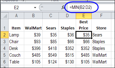
If you’re setting up a new office, or going grocery shopping, you can use Excel to compare prices. Find best price with Excel INDEX and MATCH functions, combined with MIN. This will help you calculate the lowest price for each item, and see which store sells at that price. Then, print a list, and go shopping!
Continue reading “Find Best Price With Excel INDEX and MATCH”
Screen Shots From Excel 2010
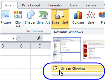
After all the fun with SmartArt charts last week, I finally noticed the Screenshot command, that’s right beside SmartArt. With the Screenshot command, you can capture an image of an entire window, or use Screen Clipping for a smaller image.
Get Rid of Number Signs in Excel
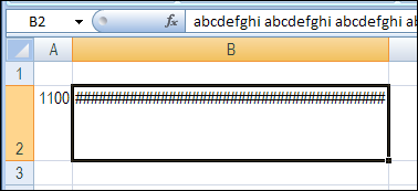
In your early days of working in Excel, you probably saw the occasional cell full of number signs (you might call them pound signs or hash marks). Here’s what you can do to get rid of number signs in Excel.