
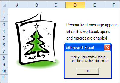
Uh-oh! It’s almost the holidays and you haven’t mailed any greeting cards yet. Don’t worry, you can create a personalized Excel message box instead! That will warm your co-workers’ hearts, and it saves paper and postage costs too.
Excel Christmas Planner
I’m just getting back from a vacation in South Carolina, where I didn’t use Excel too often, except to add up all my Christmas shopping expenses.
If you’re on my shopping list, you might be getting a basket from the Charleston market.

Or maybe you’d like some of the local barbeque sauce or a bag of grits?

Christmas Planner
There are only 10 days until Christmas, and I’m almost ready. How about you?
If you’re still planning and shopping, there is an Excel Christmas planner on the Contextures website, that you can use to help you stay organized.
The Excel Christmas planner has a budget sheet, where you can plan and track your spending.

Christmas Gift List
If you’re lucky, you don’t have too many gifts to buy. But even for a few gifts, it helps to make a list to keep track of costs.
The Excel Christmas planner helps you track your gifts too.

Christmas Tasks
The Excel Christmas planner has other sheets too, including a Christmas task list, so you can keep track of all those important things you’re supposed to do over the next few days.
You don’t want to realize on December 24th that no one has ordered the turkey!

Winter Weather
It was nice to spend some time in the warmer weather, and yes, it’s colder back here in Canada, but at least we don’t have to watch for alligators! Now I’d better go and order that turkey.

_______________
Auto Resize Excel Text Boxes
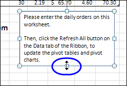
If other people will be using the Excel files that you build, it might help them if you add some instructions in a Text Box. Here are a couple of tips for setting that up.
Create Excel Chart With Shortcut Keys
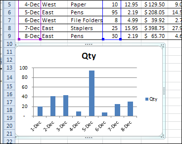
To create a chart in Excel, you can select the chart data on the worksheet, then use the Ribbon commands to insert the chart. Or, for a quicker way, you can create an Excel chart with shortcut keys. See how to insert a chart, and change an Excel setting, so it inserts a specific chart type.
Customize Excel Right-Click Menus
 Do you ever right-click on something in Excel, and the command that you wanted to use isn’t on that pop-up menu?
For example, if right-click on a cell, there is no command to turn off the gridlines.

If you can’t find the command on the right-click menu, you have to go to the Excel Ribbon or Quick Access Toolbar (QAT) instead, and try to find the command on one of the tabs there.
What commands would you add to a right-click menu? Are there commands that you added to the QAT, that would be even better in a popup menu?
Customize the Right-Click Menus
Fortunately, Doug Glancy has created a solution to the right-click menu problem, with his MenuRighter Add-in. With Doug’s free add-in, you can add commands to the pop-up menus, so the items that you need are easy to find.
The add-in is not for sissies! You need to know where the commands were on the old Excel 2003 menus – or be willing to poke around and find them.
Then, you select the right-click menu where you want to add the command, and click the buttons to add the command, and save the changes.
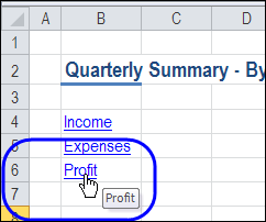
In the screen shot below, I have selected the ToggleGrid command from the Forms toolbar, and am adding it to the Cell popup menu, just above the Hyperlink command.

Find the Right Right Menu
There is a large collection of Targets, so it can be tricky to select the correct one. There are two Cell targets, so how can you decide which right menu is the right one?
While the MenuRighter is open, you can check the box for Show Labels on Menus. At the bottom of the list at the right, you can see the identity for the selected Cell target – 28-Cell.
If I right-click on cell A2, the popup menu also shows 28-Cell, so that confirms that I selected the Cell target that I want.

Use the Modified Right-Click Menus
After I added the Toggle Grid command to the Cell menu, I clicked Apply Changes, and closed the MenuRighter window.
Then, I can right-click on a cell, and turn the gridlines on or off.

It’s a command that I use frequently, so it’s very convenient to have it in the right-click menu. Thanks Doug, you made life in Excel a little easier!
Download the MenuRighter Add-in
For more instructions, and to download the MenuRighter add-in, you can visit Doug Glancy’s website: MenuRighter Add-in.
Watch the MenuRighter Video
To see the steps for adding a command to a right-click menu, by using the free MenuRighter add-in, you can watch this short Excel video tutorial.
___________________
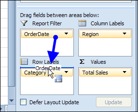
Group Pivot Table Report Filter Fields
Welcome back! The Contextures Blog was out of commission for a couple of weeks, and it’s nice to be up and running again. A few of the shingles blew off during the reconstruction, so if you notice anything missing or broken, please let me know!
Excel VLOOKUP Troubleshooting
You’re admired by your co-workers, thanks to your awesome Excel skills. Cupcakes magically appear on your desk, in thanks for your help with complex formulas.
Your boss keeps stretching the budget, to accommodate the huge bonuses you get, in reward for your amazing talents. Well, that might not be the exact situation, but I’m sure your skills are appreciated!
VLOOKUP Trouble
Then, one day, it all goes horribly wrong. Your boss needs a report in 15 minutes, and you can’t get a seemingly simple VLOOKUP formula to work.
You can see the target product numbers in the lookup table, but the formula result is #N/A, instead of the product price.

You don’t want to lose your Excel Expert badge over something this trivial, so how will you solve the problem?
Text or Number?
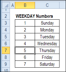
A common cause for this VLOOKUP error is that one of the values is a number, and the other is text. In this example, the lookup table codes in cell B2:B5 are stored as text values – they have a leading apostrophe.
The lookup code, in cell B8, is entered as a number – no leading apostrophe.

So, it looks like cells B2 and B8 are equal, but Excel sees them as different values.

Fix the Text Values
The easiest solution to the the VLOOKUP problem in this example is to convert the text values to numbers, so the codes in the table match your lookup values.
Or, type an apostrophe in front of your lookup code in cell B8, so it’s a text value too.
Change the VLOOKUP Formula
If you can’t fix the data, you can convert the lookup value in the Excel VLOOKUP formula. Here is the original VLOOKUP formula, that returned an #N/A error.
=VLOOKUP(B8,$B$2:$D$5,2,FALSE)
If you add an empty string to the end of the value in cell B8, the lookup number will be converted to a text string. The revised formula is:
=VLOOKUP(B8 & “”,$B$2:$D$5,2,FALSE)
This formula will also work if cell B8 contains a text value – adding the empty string won’t change the value.
More Excel VLOOKUP Troubleshooting
If this VLOOKUP formula fix doesn’t solve the problem, there are more Excel VLOOKUP troubleshooting tips on the Contextures website.
Have you run into this problem? How did you fix it?
Watch the Excel VLOOKUP Troubleshooting Video
To see the steps for fixing the Excel VLOOKUP problem, you can watch this short Excel video tutorial.
___________________
Go To Specific Part of Excel Worksheet
How can you quickly move around an Excel worksheet? In a long sheet, there’s no built-in way to go to a specific part of the Excel worksheet. Even though the sheet might print on several pages, Excel doesn’t have “page” navigation.
GetPivotData Formula Instead of Cell Link
This week, I was updating the GetPivotData Function page on my website, and remembered how hard it was to turn off that feature, in Excel 2003 and earlier.
We won’t even talk about the really olden days (Excel 2000), when you had to type those tricky GetPivotData formulas yourself!
Automatic Formulas
If you try to reference a pivot table cell, a GetPivotData formula may be automatically created, instead of a simple cell reference. This is thanks to the Generate GetPivotData feature, which is turned on by default.

The automatic formula can be a helpful feature, but sometimes you’d rather just have the cell link. You could type the link yourself, or find a way to turn off the formula feature.
GetPivotData in Excel 2003 and Earlier
In the old versions of Excel, if you want to stop that automatic formula creation, you have to add the Generate GetPivotData button to the PivotTable toolbar.
If you’re nostalgic for the old method, you can see it in the video at the end of this blog.

GetPivotData in Excel 2007 and Excel 2010
Now, it’s much easier to turn the Generate GetPivotData feature on and off.
- Select any cell in a pivot table.
- On the Excel Ribbon, under PivotTable Tools, click the Options tab.
- In the PivotTable group, click the drop down arrow for Options
- Click the Generate GetPivotData command, to turn the feature on or off.

GetPivotData Formulas
There is more information on the GetPivotData Function page, including examples of using cell references within the formula.
It’s a great way to pull specific data from your pivot tables.

Generate GetPivotData Button in Excel 2003
To see how we changed this setting in the olden days, you can watch this short video.
___________
Calculate Thanksgiving Date in Excel
Recently, Jerry Latham showed us how to use Excel to calculate the date of Easter in any year, by using a worksheet formula or Excel User Defined Function (UDF). Now, it’s getting close to Thanksgiving in the USA, so lets see how to calculate that date, with an Excel worksheet formula.