
In Excel 2007 and Excel 2010, you can use the new SUMIFS function to sum items using multiple criteria.
Use Excel COUNTIFS to Count With Multiple Criteria
In Excel 2007 and Excel 2010, you can use the new COUNTIFS function to count, based on multiple criteria.
For example, in a list of orders, you can find out how many orders were for pens, and had a quantity of 10 or more.

Page Updates
I have updated the Contextures COUNT Functions page, to include a COUNTIFS example, and video demo.
If you are using Excel 2003, or earlier versions, you can use the SUMPRODUCT function instead. There is an example for that function on the COUNT page too.
Watch the COUNTIFS Video
To see the steps for using the COUNTIFS function, you can watch this short Excel video tutorial. The written steps are on the Contextures COUNT Functions page.
There is a complete transcript of the tutorial directly beneath the video.
VIDEO TRANSCRIPT
Counting With Criteria
In Excel you can count using criteria with the COUNTIF function.
In later versions of Excel (2007 and later) you can count multiple criteria with the COUNTIFS function.
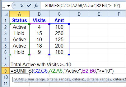
So here we have a list of items that we’ve sold and the quantity for each.
We would like to find the number of orders where a pen was the item sold and the quantity is greater than 10.
First Criteria
So in this cell I’m going to start with an equal sign and then type COUNTIFS an open bracket and the first thing I’m going to check is the item that was sold.
The range, first range is A2:A10. Then I’ll type a comma and the criteria for that range I’m just going to type in here inside double quotes pen, and then another comma.
That’s the first thing we’re going to check, is what item was sold.
Additional Criteria
Next will be the quantity so I’ll select the range that has the quantities, another comma and we want quantity greater than or equal to 10 so within double quotes
I’ll do a greater than symbol, equal, and a 10, then another double quote
Close the bracket and press Enter. There were two orders for pen where the quantity is greater than 10. Instead of typing these criteria in here I can refer to a cell.
So instead of typing pen inside double quotes, I could click on a cell where I have typed the word pen. The same for this criteria for the quantity
I’m going to take out the 10 just by deleting that, leaving the operators within the double quotes.
Adjustments
Then I’ll type an ampersand and the cell that has the number. So this is greater than or equal to whatever number is in cell E3.
When I press ENTER I get the same result. It’s just easier to change.
Then I could type a 5 here now, and we see that there were 4 orders where the quantity is greater than or equal to 5 instead of the 10 that we had in there before.
So this formula is much more flexible if you use cell references, rather than typing the values in as hard-coded values.
End Of Transcript
_________
Preparing for an Excel Expert Exam
Have you ever written an Excel proficiency exam? Maybe you’ll have some advice or tips for the person who wrote to me this week, asking for help with the Excel Expert 2007 exam.
He’s having trouble with the macros and custom functions that will be part of the test.
It’s been a long time since I wrote the Excel Expert exam, that was part of the old Microsoft Office User Specialist series. The exam has probably changed many times since then, but back then it was a mixture of multiple choice questions and simulated workbooks (if I’m remembering correctly!)
Anyway, I passed, and the certificate is still proudly displayed on my office wall. Well, it’s pinned to the wall, behind the door, but it’s still in good shape! Wow, June 1999 – that was a long time ago.

The Excel Expert Test
The Microsoft website has a list of topics that are covered on the exam, including this section on Managing Macros and User-Defined Functions:
- Record and edit a macro.
- This objective may include but is not limited to: recording a macro and editing a macro in Visual Basic for Applications (VBA)
- Manage existing macros.
- This objective may include but is not limited to: moving macros between workbooks, assigning a shortcut key to an existing macro, assigning a macro to a button in a worksheet, and configuring macro security levels
- Create a user-defined function (UDF).
Record and Edit a Macro
There are written instructions and a video on the Contextures website, for recording and testing a macro in Excel. That article briefly discusses macro security levels, and showing the Developer tab.
To see how to edit a recorded macro, you can watch the video on this blog post: Excel VBA Edit Your Recorded Macro. There are written instructions there too, in case you’d prefer to read about it.
Manage Existing Macros
If you need to copy macros into a workbook, or from one workbook to another, there are instructions here: Adding Code to a Workbook
For details on assigning a macro to a worksheet button, take a look at this page: Excel VBA Worksheet Macro Buttons. To see the code and buttons, you can download the sample workbook from that page.

______________
Hide Pivot Table Detail Without Filtering
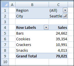
To focus on specific data in a pivot table, you can use report filters or field filters. You can also hide Pivot Table detail without filtering — use the expand and collapse buttons to show or hide details.
Continue reading “Hide Pivot Table Detail Without Filtering”
Excel UserForm Data Entry Update
Someone emailed me this week, about a problem he was having with my sample Part Data Entry UserForm.

When I took a look at the workbook, everything seemed okay, and the code had been copied and altered correctly.
Excel Named Table
Then I noticed that there was a formatted Excel table on the data collection sheet, which wasn’t in my original file.
That can cause problems if you’re using Excel VBA to add data to the first blank row on the worksheet.
Change the Last Row Code
In the comments for my Find First Blank Row blog post, Rick Rothstein suggested this code revision:
LastRow = Cells.Find(What:="*", SearchOrder:=xlRows,
SearchDirection:=xlPrevious, LookIn:=xlValues).Row
Rick mentioned that this formula ignores cells with formulas that are displaying the empty string. If your situation is such that you need to identify formula cells that might be displaying the empty string, then change the xlValues argument to xlFormulas.
Revised Excel VBA Code
So, I changed the Part Data Entry code, to use the Find method for finding the last row. I replaced this old line of code:
'find first empty row in database
iRow = ws.Cells(Rows.Count, 1) _
  .End(xlUp).Offset(1, 0).Row
With this line of code:
iRow = ws.Cells.Find(What:="*", SearchOrder:=xlRows, _
       SearchDirection:=xlPrevious, LookIn:=xlValues).Row + 1
Parts Data Entry UserForm With Combo Boxes
There is another version of the Parts Data Entry UserForm, and it’s a little fancier, with combo boxes to select parts and locations.
I’ve updated the Parts Data Entry UserForm With Combo Boxes too, with the revised last row code.

Get the Updated Sample Files
You can download the updated versions of the parts data entry forms on the Contextures website.
Parts Data Entry UserForm With Combo Boxes
_________________
Updated Excel Weight Loss Tracker
You know how tough it can be to maintain two versions of the same file. It creates twice as much work for you, and no extra rewards! So, instead of having two versions of the Excel weight loss tracker – pounds and kilograms – I’ve rolled them into one workbook.
For now, there is a separate file for the stone measurements, because it has a different layout on the data entry sheet. If possible, I’ll roll that version in later.
Excel Drop Down From List in Different Workbook
To make it easier for people to enter data, you can create drop down lists on an Excel worksheet.
Usually the source lists are stored in the same workbook as the drop downs. However, with named ranges, it is possible to use a list in a different workbook.
In the screen shot shown below, the original list is in the workbook at the left. The drop downs are in a different workbook, on the right.

There Is a Catch
My preference would be to keep the lists and drop downs in the same workbook, but if you need to have them in separate files, this technique will allow you to do that.
There’s one catch though, when using this data validation technique. The source workbook, which contains the original list, must also be open, when you are using the drop down lists.
So, it’s not a perfect solution, but it’s fairly easy to implement, as long as you remember to open the other workbook too.
Excel 2010 Instructions
I’ve just uploaded a video with instructions for this technique in Excel 2010, so you can see the steps for creating the named ranges and data validation drop down lists.
The written instructions for Excel 2007 and Excel 2010 are in this blog post: Data Validation List From Different Workbook
________________
Change All Pivot Tables With One Selection
There is a new sample file on the Contextures website, with a macro to change all pivot tables with one selection, when you change a report filter in one pivot table.
Continue reading “Change All Pivot Tables With One Selection”
Excel Pivot Table from Multiple Sheets Update
If you have similar data on two or more worksheets, you might want to combine that data in a pivot table, to show the summarized results.
Unfortunately, the pivot table from data on multiple sheets can be a disappointment.

Create a Pivot Table with Programming
A couple of years ago, Excel MVP, Kirill Lapin (KL), shared a sample file that he created, with amendments by Hector Miguel Orozco Diaz.
It uses code to automatically create a pivot table from multiple sheets in a workbook.
You can read the details here: Create a Pivot Table from Multiple Sheets.
Revised Solution
Kirill’s sample file was created as a conceptual prototype, and targeted advanced VBA users. The code has minimal error handling and compatibility checks.
However, the sample file was extremely popular, and Excel users at all skill levels wanted to adopt this solution in their own applications. To make things easier, Kirill has created a similar solution based on ADO.
Advantages:
- No need for temporary file generation
- The code is faster and less prone to errors
Disadvantages:
- No manual refresh of the PivotTable
- Need to rebuild connection from the scratch to update the cache with new data
Download the ADO Sample File
You can download the new ADO version of the file from the Contextures website: PT0024 – Pivot Table from Multiple Sheets – ADO version.
There is also a “Plug and Play” version of the file, at the same link.
________________
Change Excel Comment Shape
When you insert a comment in Excel, a rather boring yellow rectangle appears, where you can add your text.

That’s all very proper and dignified, but sometimes you want something a bit more attention-getting.

In the good old days of Excel 2003, it was easy to change the comment shape, with a simple right-click. In Excel 2007 and Excel 2010, you need to add a command to the QAT, so you can change the comment shape.
Add the Change Shape Command to the QAT
- At the right end of the QAT, click the drop down arrow
- Click More Commands
- In the Choose Commands From drop down, click All Commands

- In the list of commands, click Change Shape, and click Add, to move it to the Quick Access Toolbar

- Close the Excel Options window.
Change the Comment Shape
- Right-click the cell which contains the comment.
- Choose Edit Comment
- Click on the border of the comment, to select it.

- On the QAT, click the Change Shape command, and click on a shape to select it.

- If necessary, drag the corner handle of the comment, to adjust its size, to fit the text.
- When finished, click outside the comment.
Watch the Video
To see the steps for adding the Change Shape command to the QAT and changing the comment shape in Excel 2010 or Excel 2007, you can watch this short Excel video tutorial.
_____________________